1. Introduction

This workshop’s objective is learning to use onesait Platform’s different components to perform completely an information analytics process flow, from the ingestion, through the ML, to the visualization.

The starting point is a dataset in the Kaggle platform https://www.kaggle.com/mylesoneill/game-of-thrones along with kernels from it https://www.kaggle.com/shaildeliwala/exploratory-analysis-and-predictions and https://www.kaggle.com/zhy450324080/death-prediction-battle-analysis.

It is made up of the following steps: 

• Data ingestion and preparation:
• Creation of the ontologies with which we will work.
• Creation of an DigitalClient to access the ontologies.
• We will have three information ingest types:
1. Import tool
2. Dataflow
3. Notebook
• Data analytics & exploration & ML on the loaded data using the platform’s notebooks.
• Visualizing the data using the platform’s dashboards.

For this workshop, we will use to following datasets:

• character-predictions.csv to be loaded form Control Panel’s Import Tool.
• battles.csv loaded from the DataFlow component.
• character-deaths.csv loaded from the Notebooks component.

We are assuming programming experience (particularly in Python) and having performed the IoT workshop previously, meaning that basic concepts on the platform will not be explained.
This workshop requires a CloudLab environment user with Analytics Role.

2. Information Ingestion

In this chapter, we will perform the dataset file ingestion through different tools, all of them included in the platform, each appropriate to some fields.

Isolated load from Import Tool

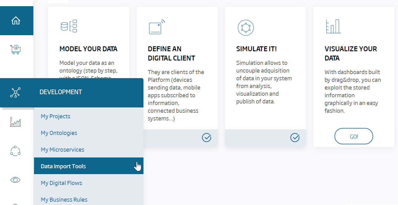
The Platform’s Import Tool provides an easy way to create ontologies inferring the data schema from json, csv, xls, xlsx or xml files, then loading them automatically. It can also be used to load data in an existing ontology, or to create an empty one.
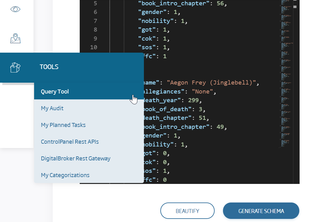
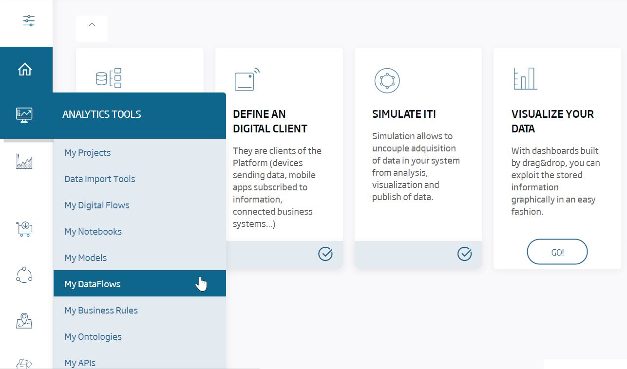
The first step for an already-logged analytics user is accessing its menu:

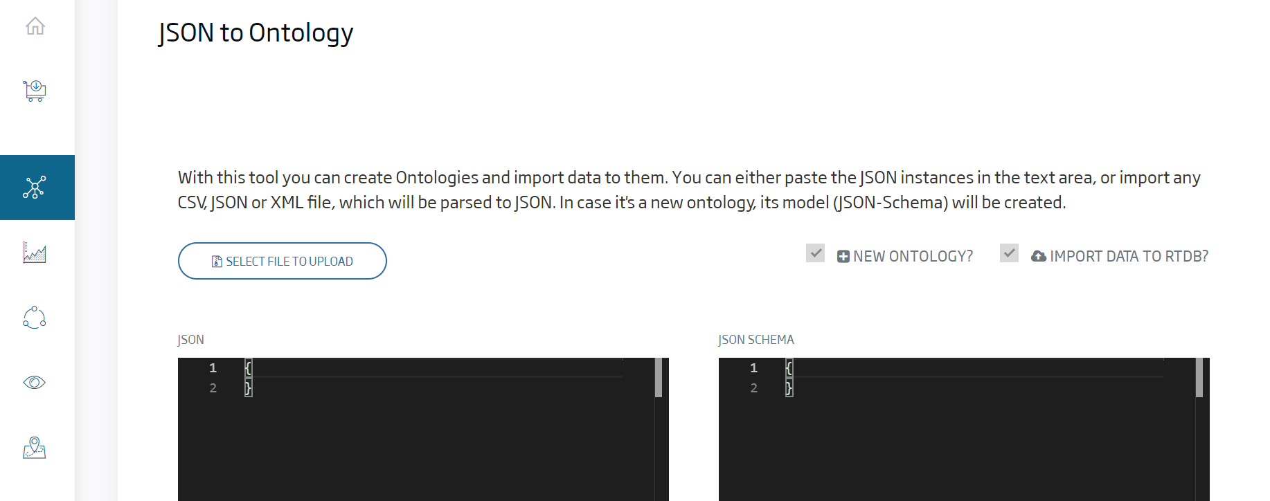
There we see a simple interface with two main columns: To the left, the data (or a summary of these) to be loaded; to the right, the inferred schema.
We select the file to upload as an ontology. In our case, it will be this one:

To download it, we can double-click on it, then save it in some folder. This same file will be the one we select when we click “Select File To Upload”.

As you can see, the csv has been red and correctly transformed to JSON format. The next step will be clicking on “Generate Schema”, and then we can see the ontology schema that the tool automatically inferred.

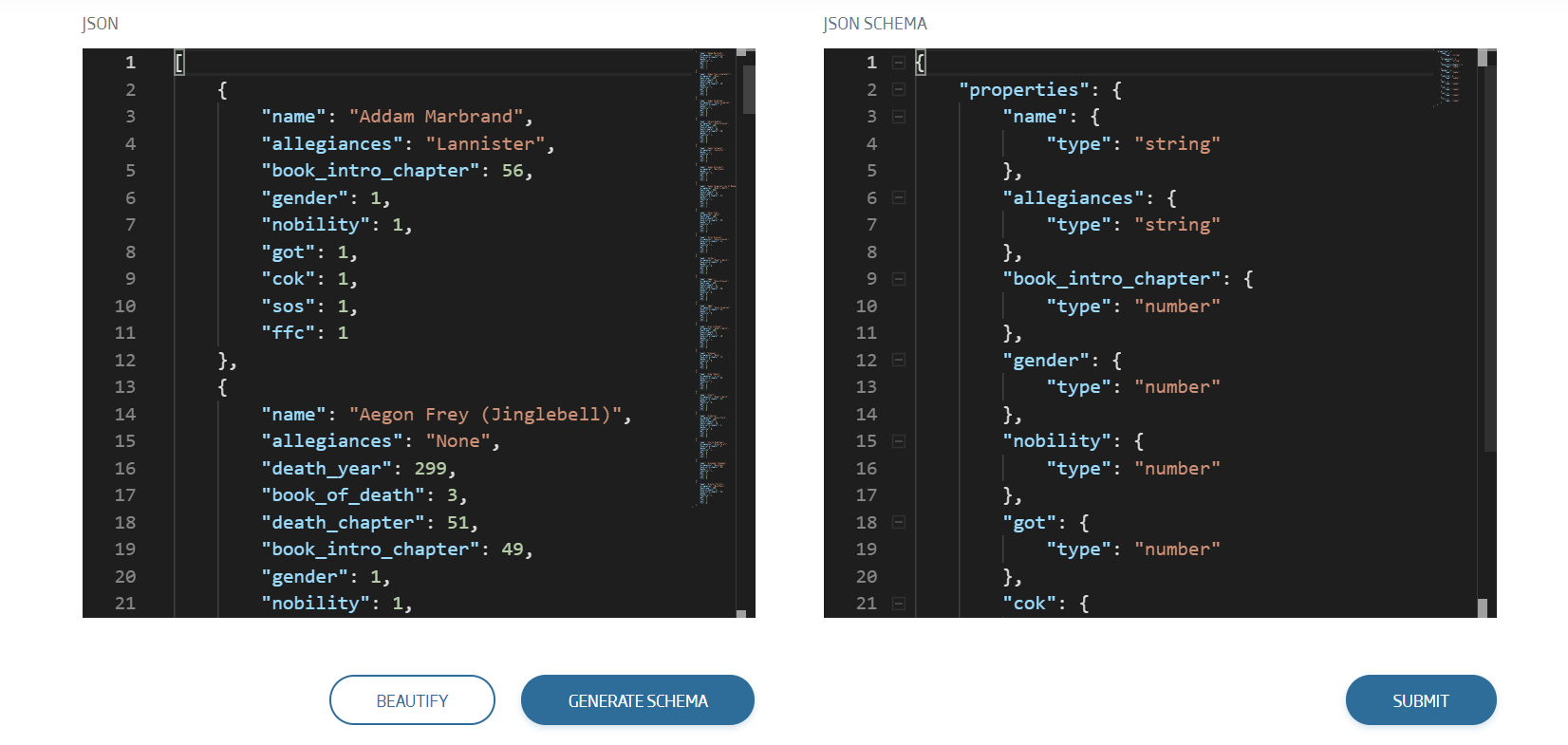
The last step in this section, having checked both New Ontology and Import Data To RTDB:

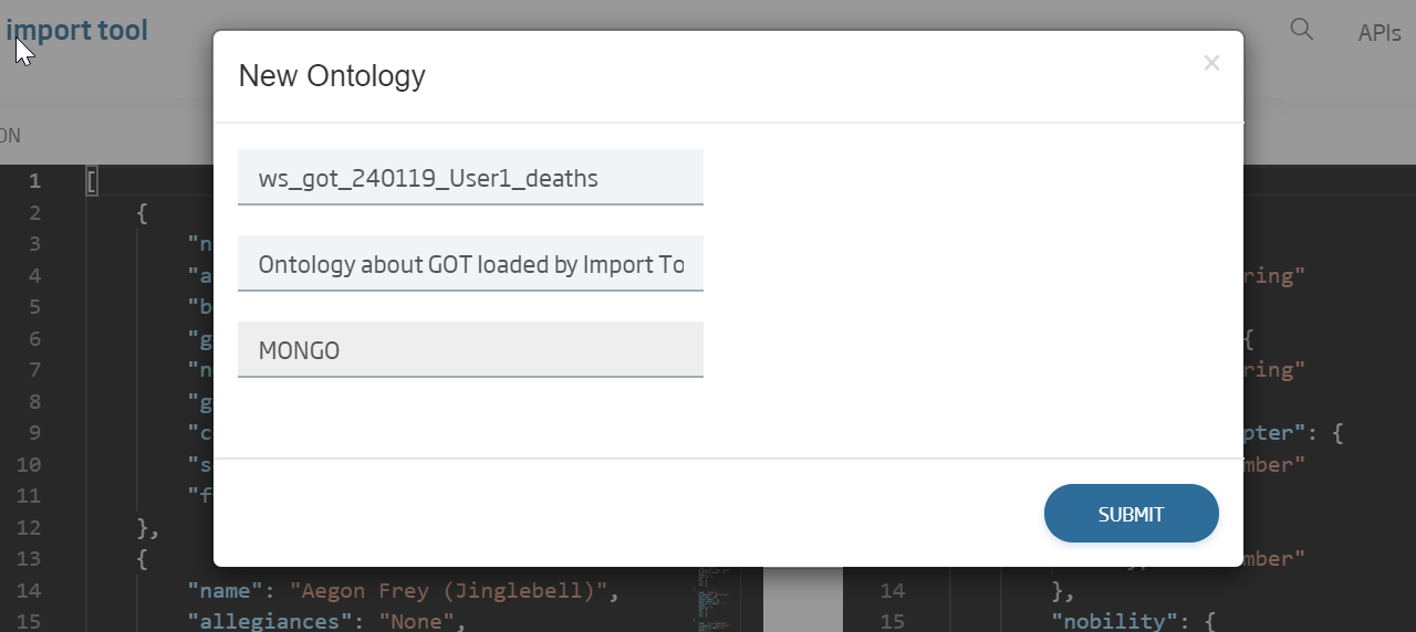
We click Submit, in the lower part, and we will see a pop-up to insert the ontology’s name, its description and the database it will use. It is important to have an ontology name of your own, because the platform does not allow two ontologies with the same name:

• Name: ws_got_{date}_{user}_deaths
• Description: Whatever the user wants.
• Datasource: MONGO

A progress bar will show the load status. When it is finished, we will be notified.
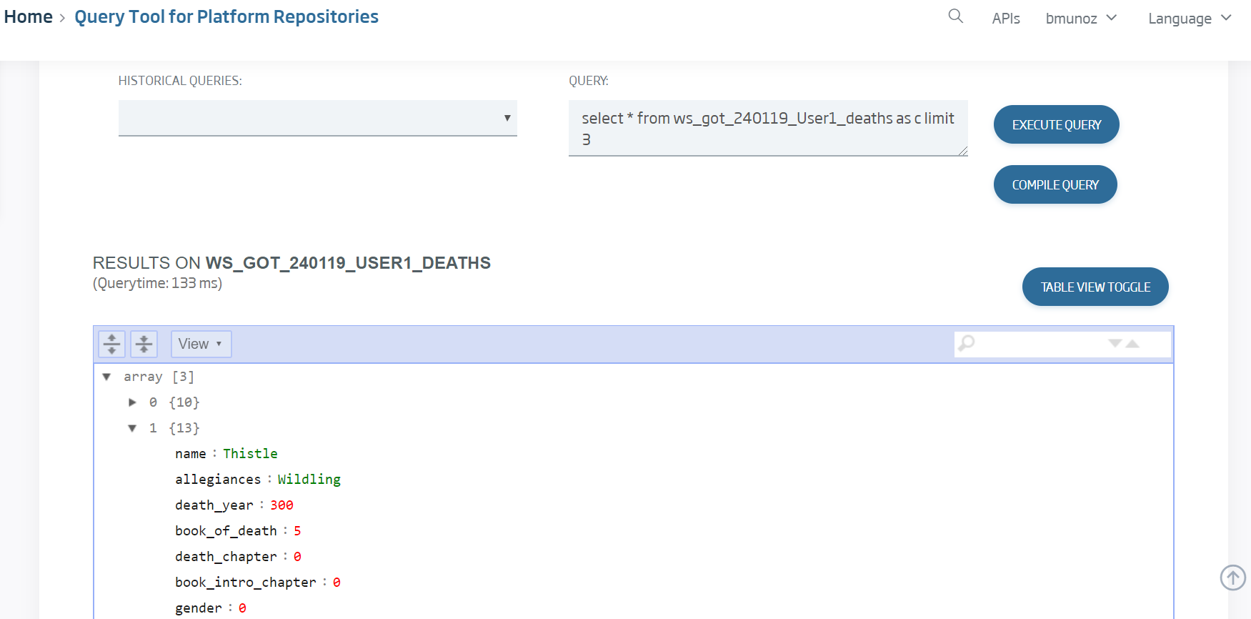
To see all the data that have been loaded, we can go to the Query Tool and launch the default query we have:

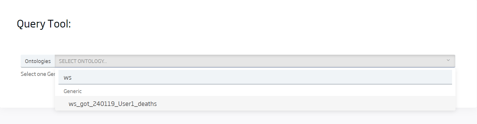
Select the ontology we have just created, then load:

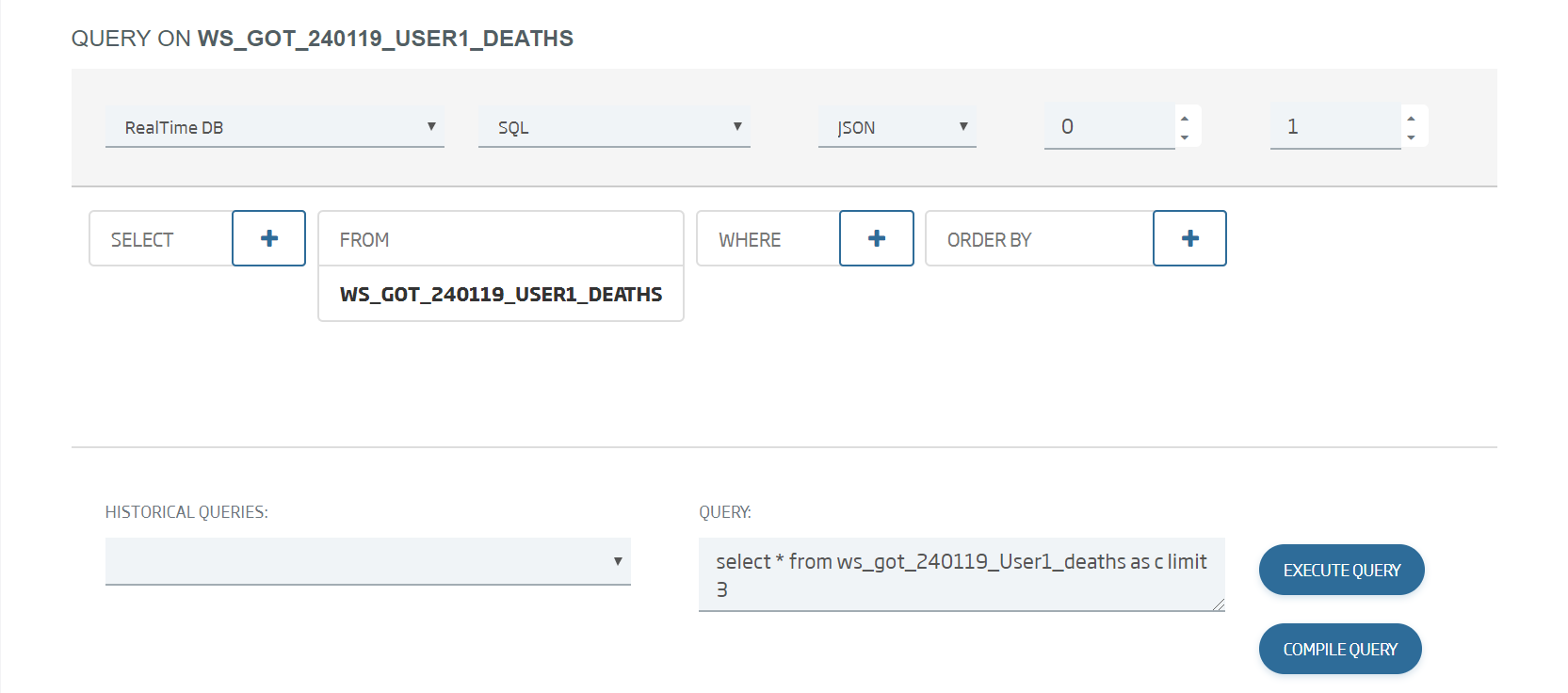
Finally we launch the generated default query with “Execute query”:

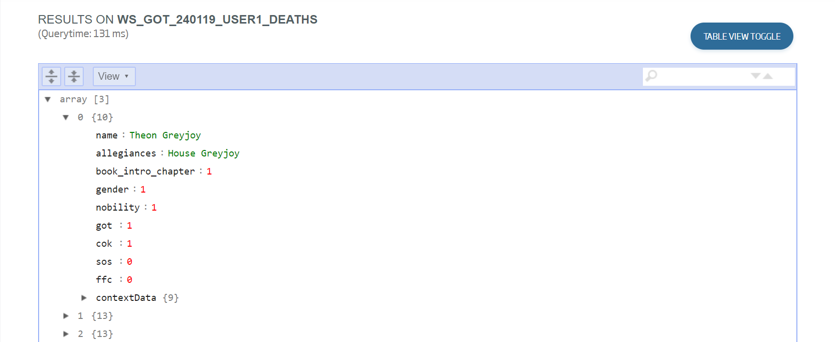
We can see that, for every instance, the loaded data correspond to a row in the initial csv. We can also see that, if a field is not included in the row, it does not reach the target ontology.

ETL/Streaming from Dataflow tool

The Dataflow tool is based on the open-source software, Streamsets (https://streamsets.com/).

This tool allows visually modelling ETLs and data streaming flows, and also controlling them, see their logs, etc.

The data will enter through a single selected origin, and can go to one or several destinations. Among many, the Platform itself is allowed both as an origin and as a destination, using the corresponding "onesait Platform" node.
In this case, we cannot automatically infer the schema, meaning that we must create both an ontology and an associated Digital Client (These steps are not described, because this knowledge from the IoT workshop is assumed).

The target ontology data are these:
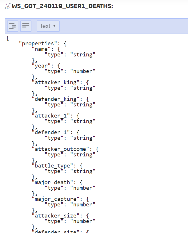
Name: ws_got_{date}_{user}_battle
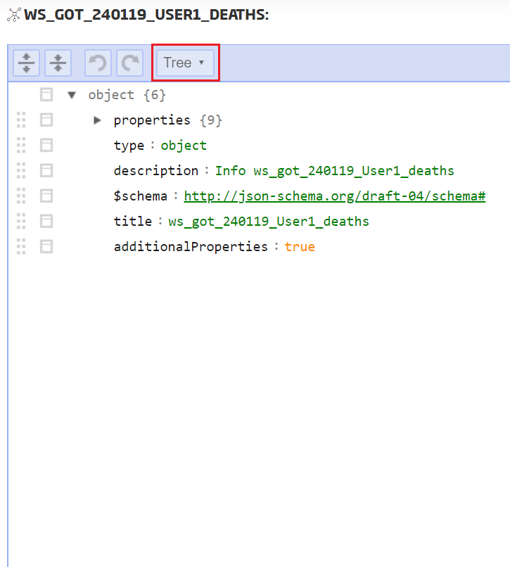
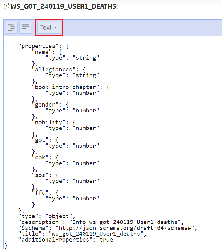
Schema: General > EmptyBase (once selected, click Update Schema and paste the following schema)

Schema (include when creating the new ontology):

{
"properties": {
"name": {
"type": "string"
},
"year": {
"type": "number"
},
"attacker_king": {
"type": "string"
},
"defender_king": {
"type": "string"
},
"attacker_1": {
"type": "string"
},
"defender_1": {
"type": "string"
},
"attacker_outcome": {
"type": "string"
},
"battle_type": {
"type": "string"
},
"major_death": {
"type": "number"
},
"major_capture": {
"type": "number"
},
"attacker_size": {
"type": "number"
},
"defender_size": {
"type": "number"
},
"attacker_commander": {
"type": "string"
},
"defender_commander": {
"type": "string"
},
"summer": {
"type": "number"
},
"location": {
"type": "string"
},
"region": {
"type": "string"
},
"note": {
"type": "string"
},
"attacker_2": {
"type": "string"
},
"attacker_3": {
"type": "string"
},
"attacker_4": {
"type": "string"
},
"defender_2": {
"type": "string"
},
"defender_3": {
"type": "string"
},
"defender_4": {
"type": "string"
}
},
"type": "object",
"description": "Info workshop_got_battle",
"$schema": "http://json-schema.org/draft-04/schema#",
"title": "ws_240119_User01_battle",
"additionalProperties": false
}

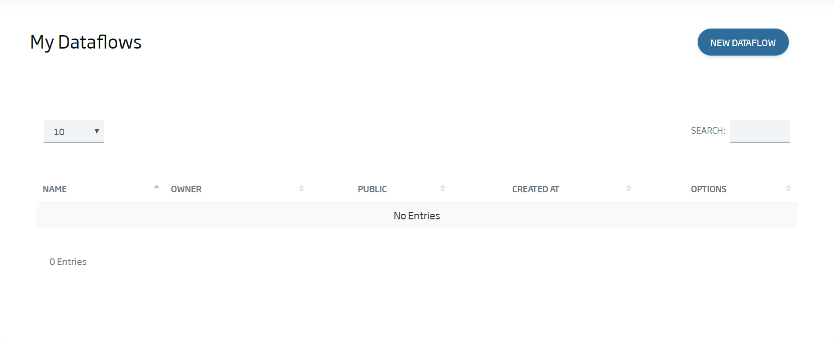
Once we have created the ontology and an DigitalClient to access it, we must create our first DataFlow: 

We will see the list of DataFlows, and we have to click in the upper right part to create one. 

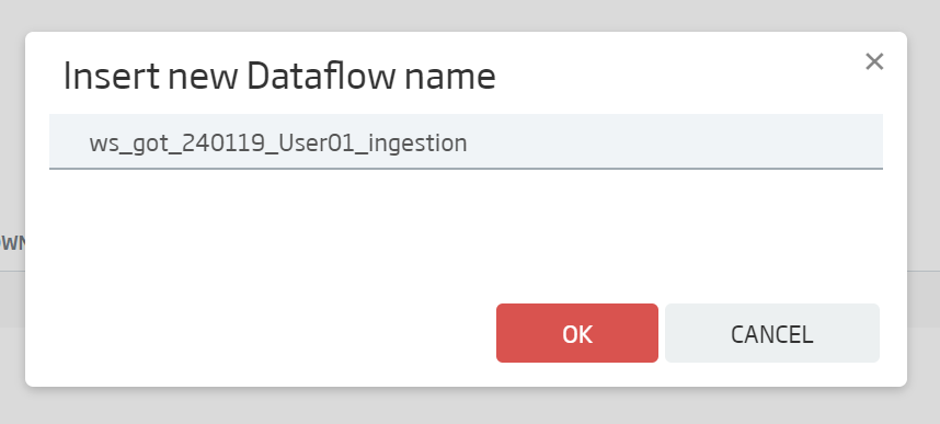
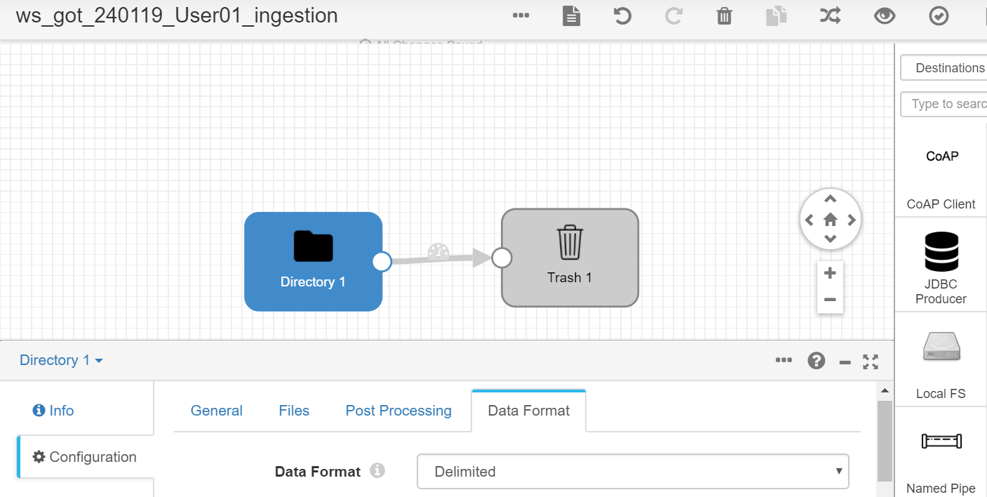
We name it: ws_got_{date}_{user}_ingestion y and click OK.

Once the canvas loads, we can see its edition screen.

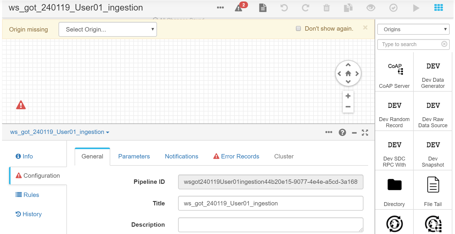
Using the element palette to the right, we can start building our flow.
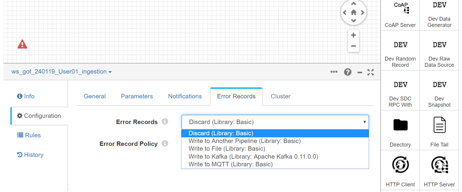
The first step is solving one of the mistakes we see in the screen: The way the current pipeline deals with error records. To do this, go to the Error Records tab and select Discard, because we don’t want to do anything with those records should they exist.

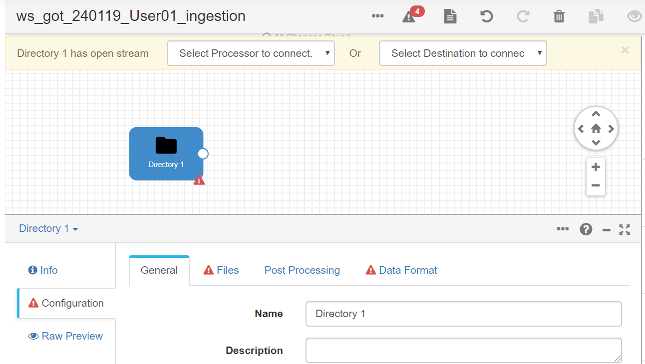
Having solved this, we now will include our data origin.

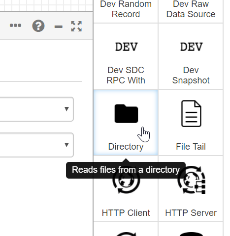
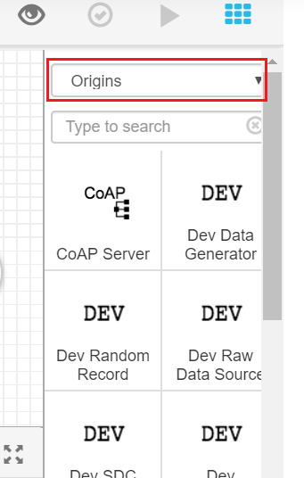
In this case, we have the Dataflow component’s container path, a shared volume with the data we want to ingest, in a UNIX file system path. To ingest this data file, we will use the “Directory” origin among the Origins. Drag and drop it to have it in the canvas.

 
We configure the origin path with:
/data/workshop
And we place the file directly in the file pattern:
battle.csv

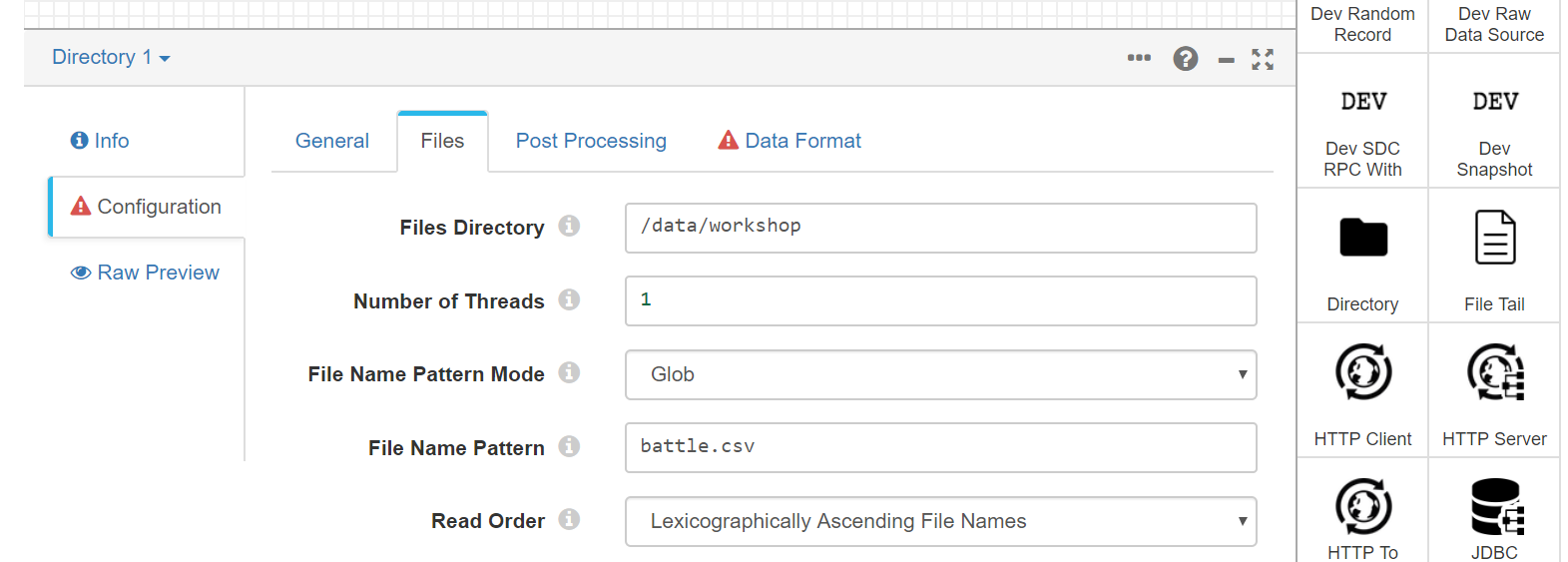
It's a standard csv file with comma separations and header. This is why we now specify this format in the Data Format tab (under Configuration).

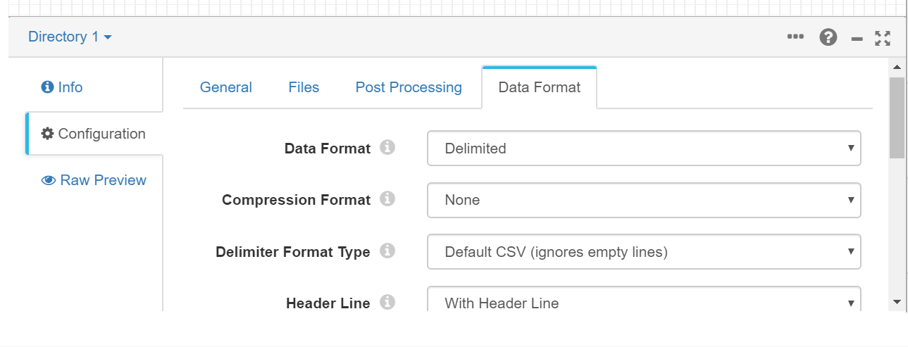
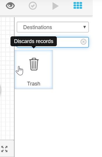
As it is a standard file, we don’t have to specify more than that, except that we want to use its header (With Header Line), so that we go to the flow start. This wouldn’t be possible without a destination, so we use, in debug mode, the Destination "Trash" and we connect it to our origin, "Directory 1". By linking both, we should get no errors in the flow: 

So we can go to validate it and see that the flow is ready to start:

If this is correct, we will be notified. Later, we will check the data entering the flow so that, instead of starting it, we will preview it: 

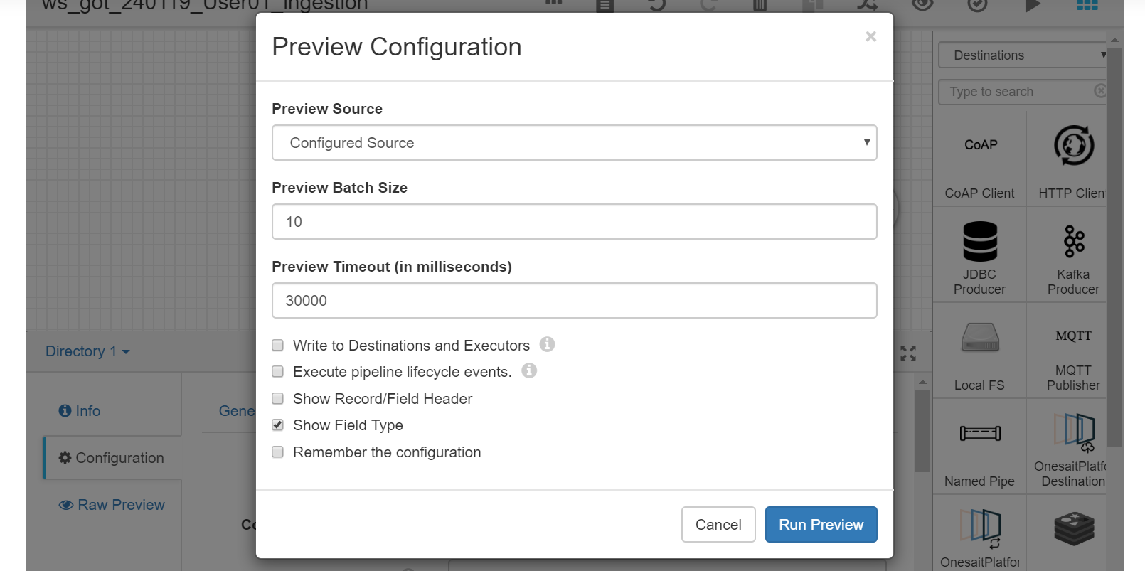
With the default parameters, we select Run Preview:

We can see that the fields are structured in records and how these change every step of the process. This means we can visually refine our flow. 

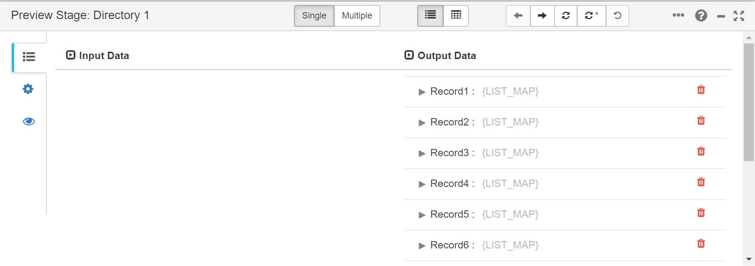
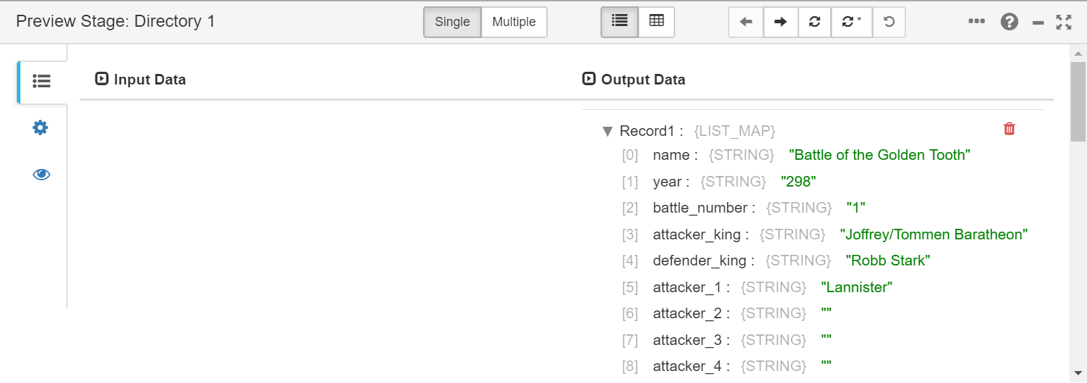
Once we have seen how we can refine and see our flow, we will complete it.

If we see the structured returned by Directory, we can see that the battle_number field is not needed, and that every fields are String type, so that we need to convert some of them to integer so they can be correctly ingested. We also see that there are fields that are empty so that, for the sake of simplicity, we will replace them with -1 in every case. 

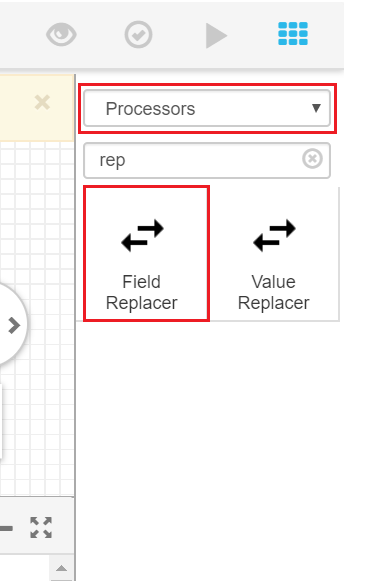
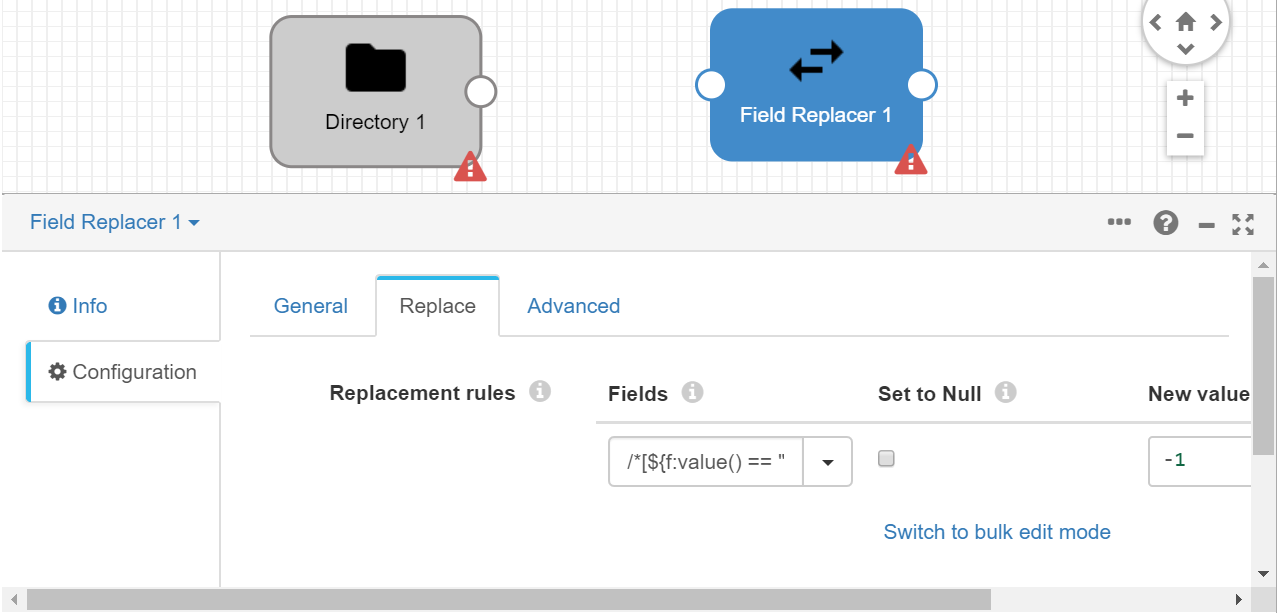
First, we will include a new stage in our flow to convert empty fields to -1. This will be possible thanks to the "Field Replacer" Processor. In this case, to do it massively, once added, we will include this in the Replace tab:
/*[${f:value() == ""}]
and specify that the new value is -1.

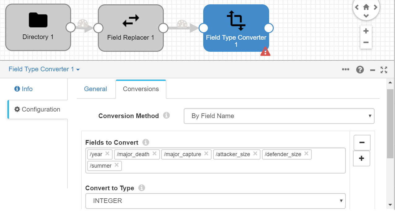
The next step is converting the number fields to Integer format. To do this we will use another processor, "Field Type Converter".
Before any further configuration, we will join the three elements in order, so that, thanks to this, field selection in the last added element will be easier. We go to the Conversions tab and include the following fields, to Integer format (If they are not listed, remember to include a /slash before each field):

• year
• major_death
• major_capture
• attacker_size
• defender_size
• summer

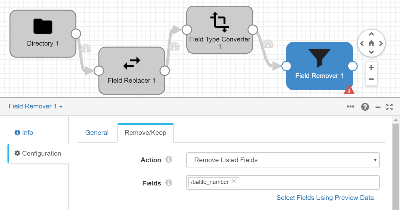
As the next-to-last step, we will remove the battle_number field because our ontology does not have it and we don’t feel it’s needed. We do this with the "Field Remover":

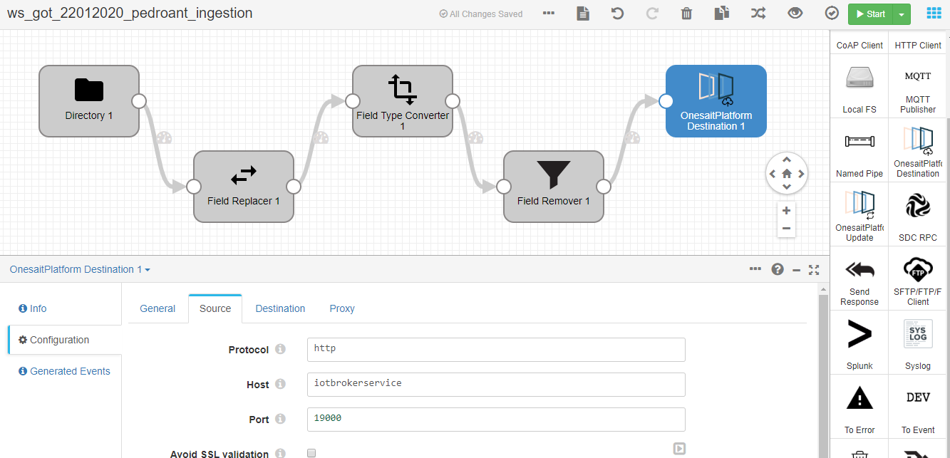
Finally, we will include, as the destination, the platform node in under "destinations" with the name "Onesaitplatform Destination". We configure it like this:
Protocol: http
Host: iotbrokerservice
Port: 19000
Token: (the token generated by the Digital Client for the ontology we had created and associated to it)
IoT Client: Name of the DigitalClient we had created

IoT Client ID: We can leave the default autogenerated one
Ontology: Name of the ontology we had created 

In the component’s Destination tab, we’ll leave the default values.

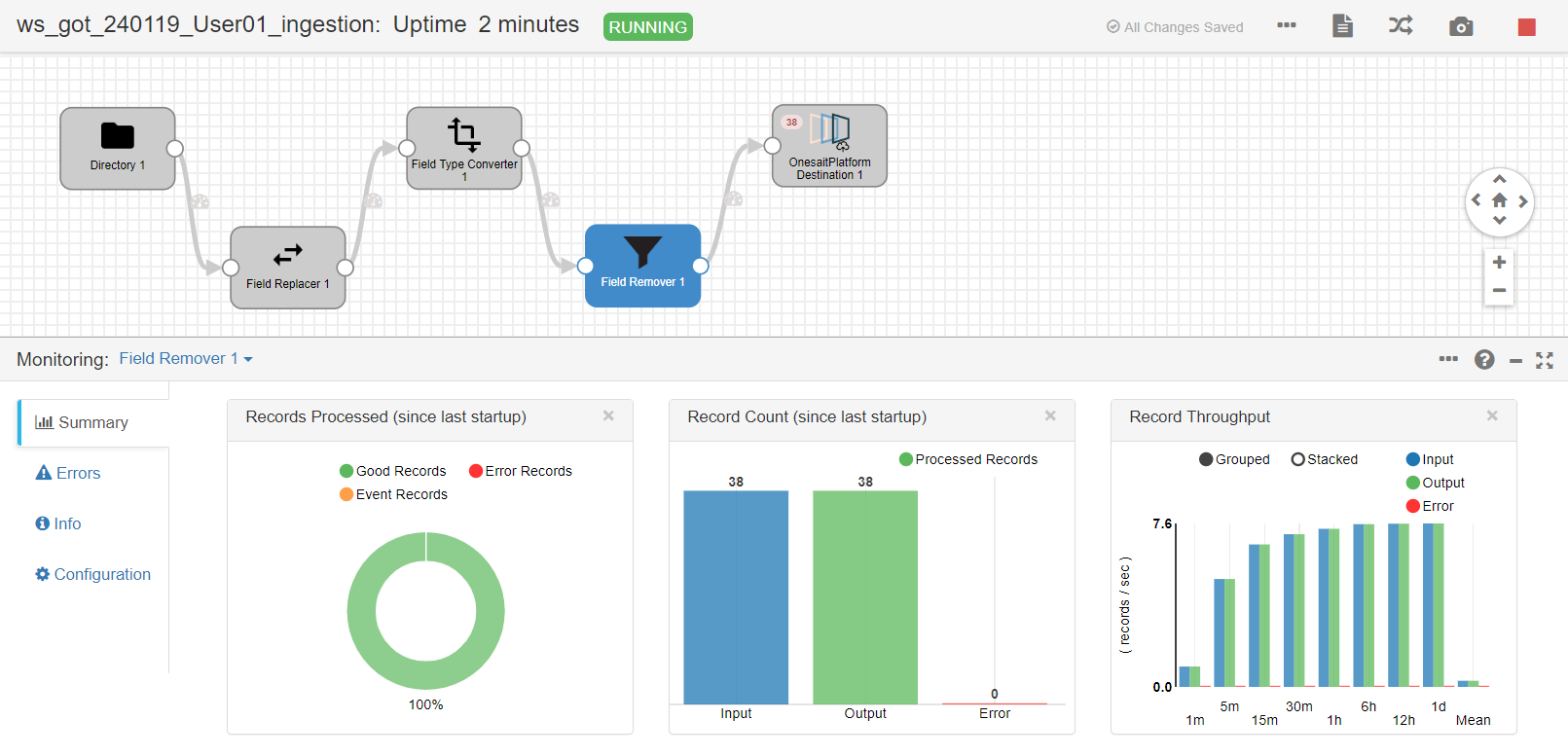
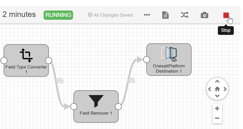
Finally, we will start the flow and we can see in real time the progress of ingestion, load throughput, number of total records or error records, etc.

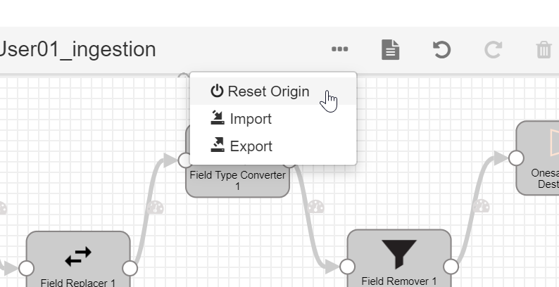
If we have accidentally launched the flow and we see it is not loading data, we can reset the origin in the we see. This is because Streamsets keeps a cursor on the last read file and the position, to avoid duplicated readings.

Now we can verify with the Query Tool that the load process was correct.

Once this section is done, and the data is loaded, the flow will be stopped with the Stop button:

Load from the Notebooks for Data Scientists

This section will serve as an introduction to the Platform’s Notebook tool and to the following section.

The first thing we will do will be uploading a file to the platform’s My Files tool.

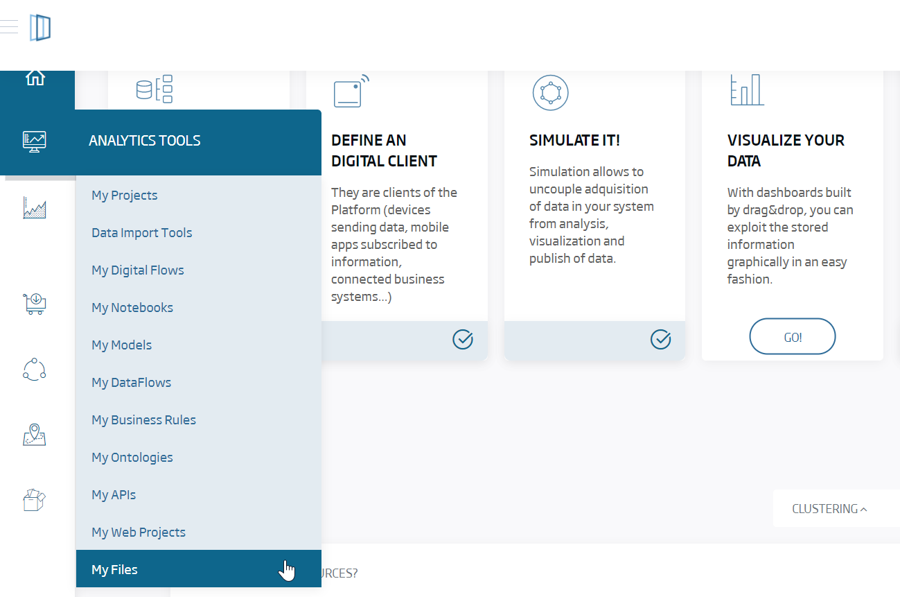
With this tool, we make files available in a simple, secure way, via URL, and we can manage them from the platform, use them from third parties and other Platform’s components such as the notebooks. 

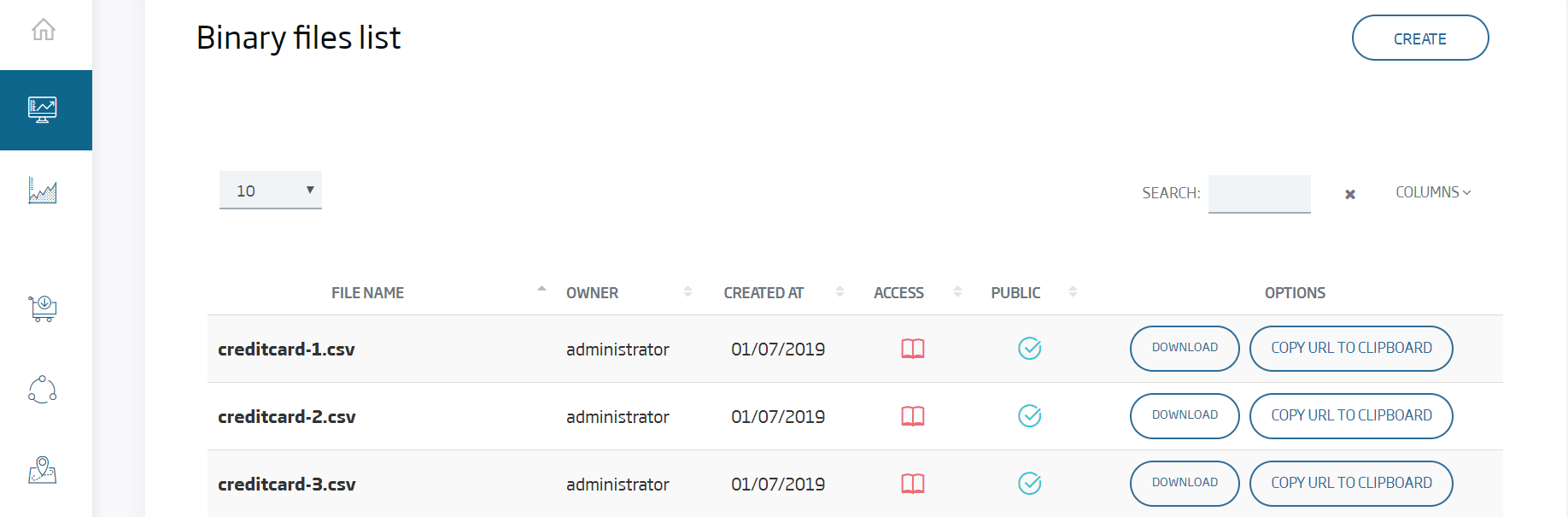
We click Create and select the next file that we must have downloaded to our computer, we leave the default values for the other parameters, and then Submit.

With this, the file will appear in our list.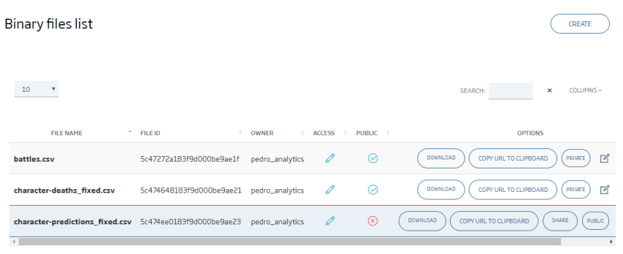 

 

Lastly, for the sake of simplicity, will be selecting public so that the file is public and can be read without authentication.

Once we’ve done this, we can click "Copy URL to Clipboard" because we will need in the following steps.

Now we are going to create our first Notebook in the platform. This ecosystem is based on Apache Zeppelin’s last version (https://zeppelin.apache.org/). It provides with notebooks for analytics, online viewing, algorithm execution and many other options in a multi-user, collaborative, versioned, executable environment, either remotely, punctually or temporized, with control and the capacity to execute different programming languages and communicate them with each other.

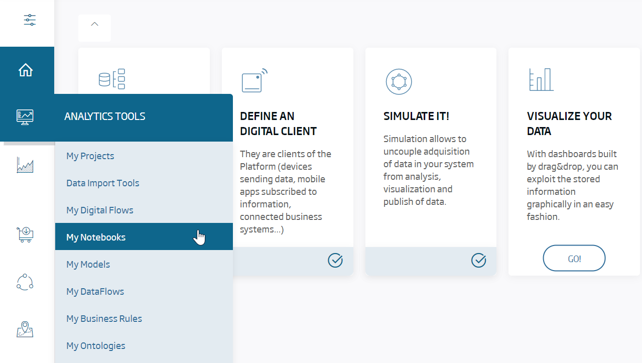
It is made up of paragraphs. Each of these includes an "interpreter" noted %interprete. Each interpreter type has different assignation, including executing a specific programming language such as Python, Scala or R; or launching queries against a database, a SparQL, Neo4J, executing Shell commands or painting HTML in the user’s screen. To understand it, nothing better than see it in action. Go to My notebooks and select Create new notebook:

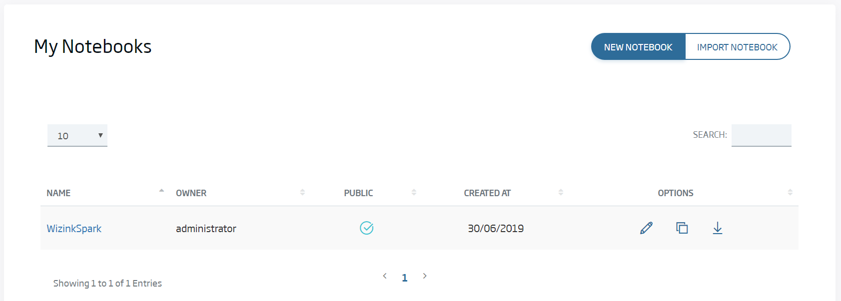
We name it ws_got_{date}_{user}_analytics and, when we create it, we will see the following screen: 

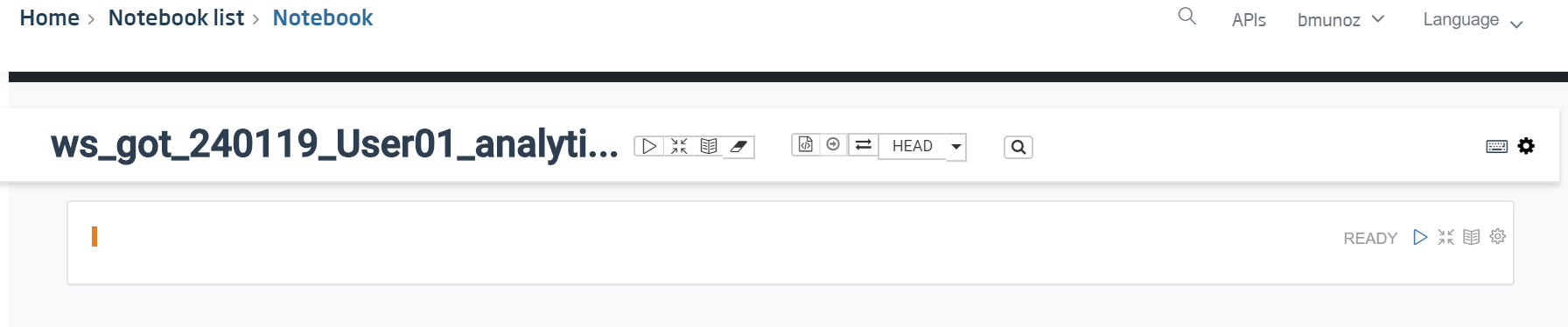
Our goal will be, using Python language and the pandas library (Python’s dataframe library), load the file we had previously uploaded to the platform as a dataframe, then insert it in the platform with a new ontology.

In the next section, we will use this dataframe for inline viewing and ML algorithms.

Firstly, we will create this last ontology and associate it to our DigitalClient. The name and schema are the following ones. It is created exactly as the previous one in the Dataflow exercise.

Name: ws_got_{date}_{user}_cdeads
Schema:
{
"properties": {
"sNo": {
"type": "number"
},
"actual": {
"type": "number"
},
"pred": {
"type": "number"
},
"alive": {
"type": "number"
},
"plod": {
"type": "number"
},
"name": {
"type": "string"
},
"male": {
"type": "number"
},
"mother": {
"type": "string"
},
"father": {
"type": "string"
},
"heir": {
"type": "string"
},
"book1": {
"type": "number"
},
"book2": {
"type": "number"
},
"book3": {
"type": "number"
},
"book4": {
"type": "number"
},
"book5": {
"type": "number"
},
"isAliveMother": {
"type": "number"
},
"isAliveFather": {
"type": "number"
},
"isAliveHeir": {
"type": "number"
},
"isMarried": {
"type": "number"
},
"isNoble": {
"type": "number"
},
"numDeadRelations": {
"type": "number"
},
"boolDeadRelations": {
"type": "number"
},
"isPopular": {
"type": "number"
},
"popularity": {
"type": "number"
},
"isAlive": {
"type": "number"
}
},
"type": "object",
"description": "Info workshop_got_cpred",
"$schema": "http://json-schema.org/draft-04/schema#",
"title": "workshop_got_cpred",
"additionalProperties": true
}

With this ontology created and associated to the Digital Client, we go back to our notebook.

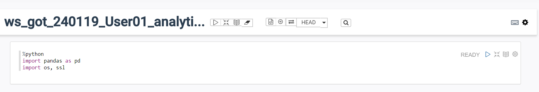
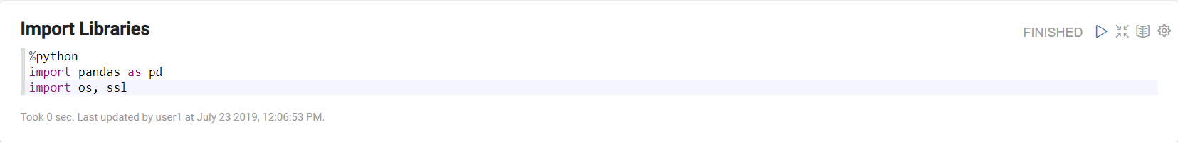
As we can see, we have the cursor in the first paragraph. The first thing we must do is importing Python’s pandas library, meaning that %python must precede the first paragraph.

%python
import pandas as pd
import os, ssl

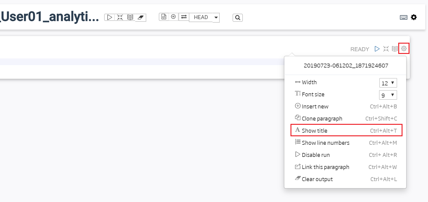
To organize our work, we give a title to the paragraph, to remember what it does if we have to use it again.  

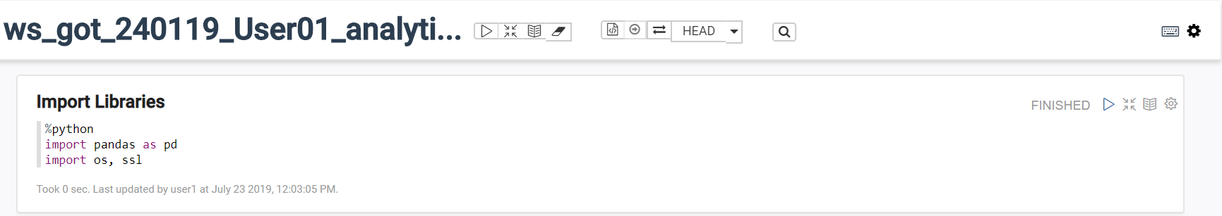
As we can see, we are going to use a couple more libraries, os and ssl, which will help us non-securely accessing the file.

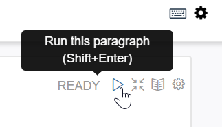
We can already execute this paragraph with the (Play) button to the right of it, or with the cursor itself on it and shift+enter. We see that it changes almost instantly from Ready to Finished status, denoting the paragraph execution end.

In the next paragraph, also Python, we will load in a pandas dataframe’s remote file’s line.
We add a new paragraph with the title: load cdeath file into pandas:

%python
if (not os.environ.get('PYTHONHTTPSVERIFY', '') and
    getattr(ssl, '_create_unverified_context', None)): 
    ssl._create_default_https_context = ssl._create_unverified_context
character_deaths = pd.read_csv("url from file")

and execute it:

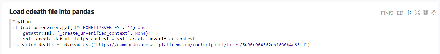
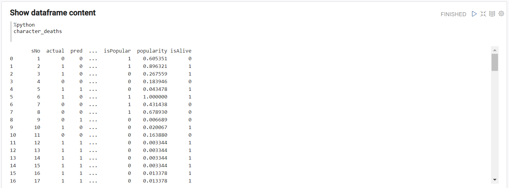
If there is no error, then the file was correctly loaded. The first three lines are to switch off Python’s ssl authentication and prevent a certificate error. We must correctly include the public file’s url we had uploaded. If we want to see the data, we only need to write the dataframe’s name (character_deaths) in a third paragraph and execute it.

Lastly, as for now our goal is inserting data in the platform, we will transform this pandas dataframe into a valid JSON. We remove the NA data and leave those compatible with the ontology. In the second line, we include this JSON String in a Zeppelin context variable that will be used to communicate between languages:

%python
character_deaths[['sNo','actual','pred','alive','plod','male','dateOfBirth','dateoFdeath','book1','book2','book3','book4','book5','isAliveMother','isAliveFather','isAliveHeir','isAliveSpouse','isMarried','isNoble','age','numDeadRelations','boolDeadRelations','isPopular','popularity','isAlive']] = character_deaths[['sNo','actual','pred','alive','plod','male','dateOfBirth','dateoFdeath','book1','book2','book3','book4','book5','isAliveMother','isAliveFather','isAliveHeir','isAliveSpouse','isMarried','isNoble','age','numDeadRelations','boolDeadRelations','isPopular','popularity','isAlive']].fillna(-1)

character_deaths[['name','title','culture','mother','father','heir','house','spouse']] = character_deaths[['name','title','culture','mother','father','heir','house','spouse']].fillna("")
jsondataframe = character_deaths.to_json(orient="records")
z.z.put("instances",jsondataframe)

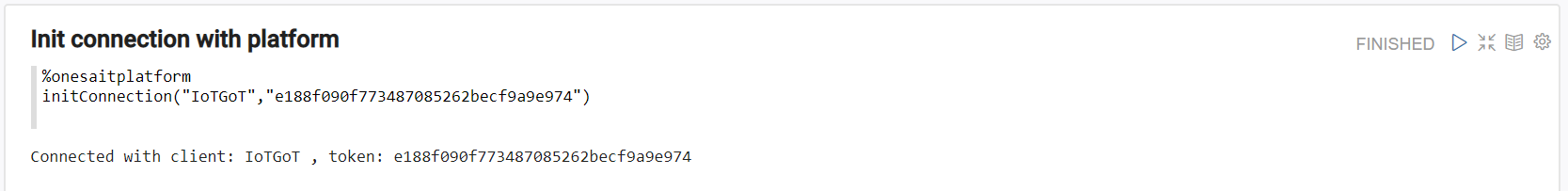
To interact with the platform, we have the %onesaitplatform interpreter. To start this interaction, the first thing we need is starting a connection with the platform this way:

%onesaitplatform
initConnection("IoT Client","Access token")

So that, if our parameters are correct, we can access our ontologies by executing this. For security reasons, connection ends in a few minutes, so that, if other instructions in the platform cause problems, you may need to execute the paragraph again 

Lastly, as we are connected to the platform, we also execute, with onesaitplatform interpreter, and also thanks to Zeppelin context, we insert data in the destination ontology:

%onesaitplatform
insert("{nueva ontologia creada}",z.get("instances"))

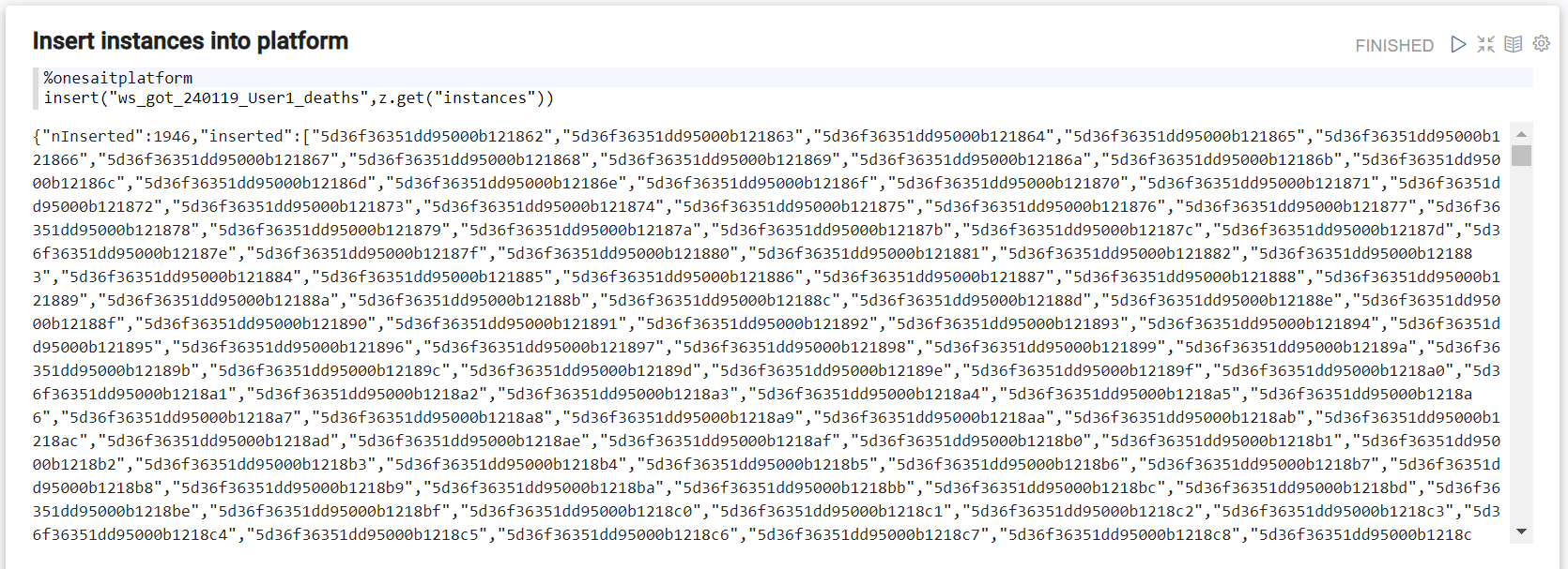
We can check, using Query Tool again, that our ontology has loaded the data.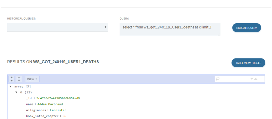

3. Data analytics & exploration & ML on loaded data through the platform’s notebooks

In this section, we will briefly explore the data we loaded in the character_deaths dataframe.
Starting with the already-created notebook, we can start seeing the data it contains. Firstly, we will use a new interpreter (markdown) to write HTML easily and delimit sections. The # means h1 in HTML, that is to say, big heading text.

Now we will start adding several %python paragraph to see the dataframe
Dataframe length:

%python
character_deaths.size

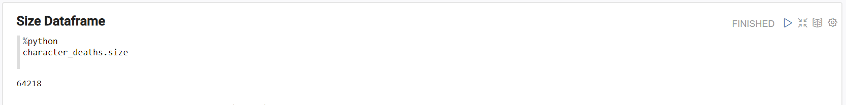
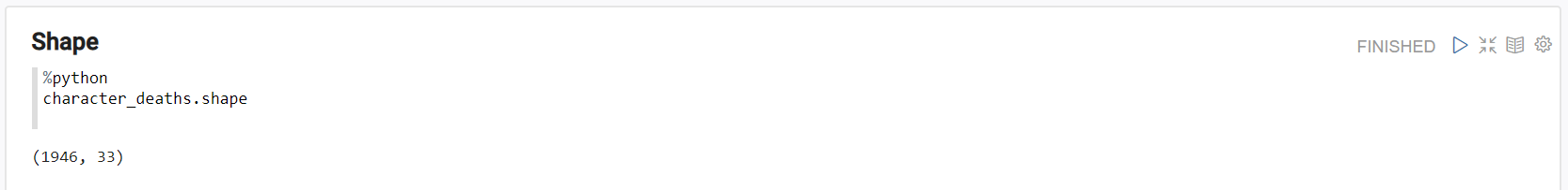
Its size
%python
character_deaths.shape

 
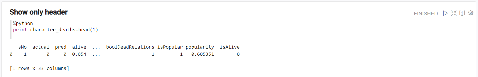
Show only header
%python
print character_deaths.head(1)

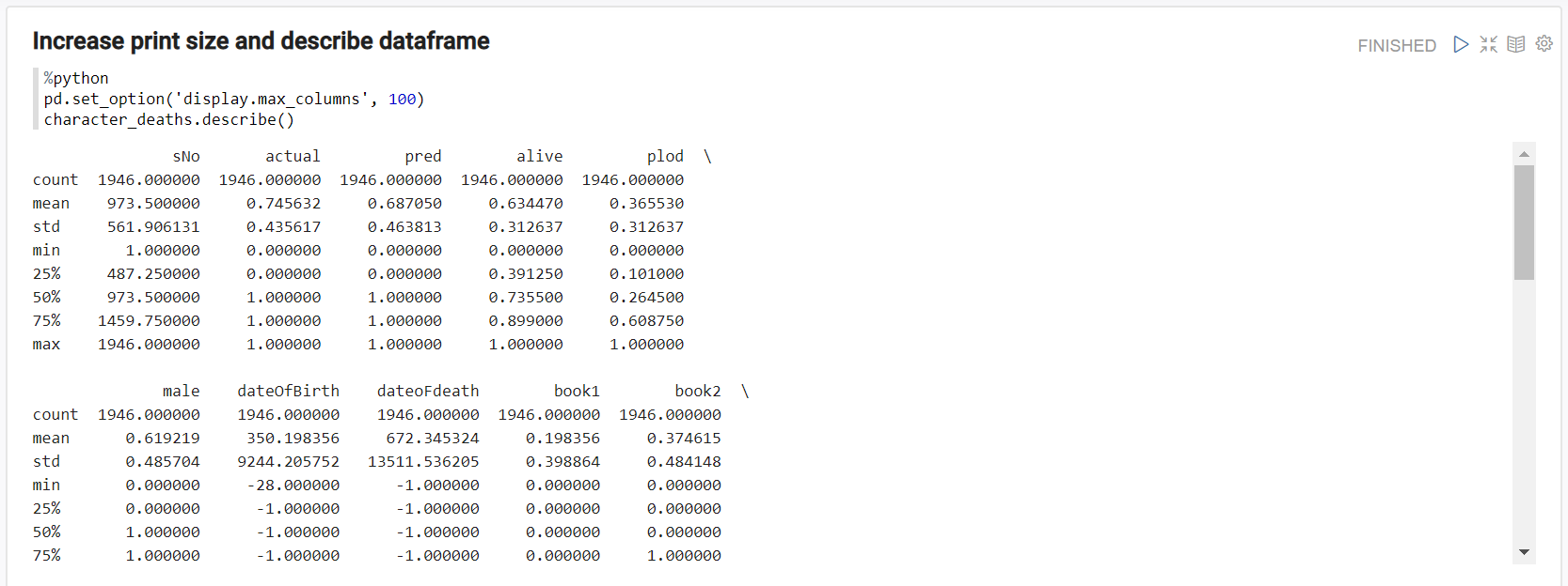
Increase maximum number of visible columns and see statistic data of each column  
%python
pd.set_option('display.max_columns', 100)
character_deaths.describe()

We can do any number of Python transforms, processing and viewings with pandas, even joining a dataframe with another one.
Now we will use the SQL engine on notebook pandas with %python.sql, to instantly graph the data as if it was a database. We only need to define a variable to be dataframe, in our case character_deaths , then launch queries on it asking questions:
Most popular characters by house
%python.sql
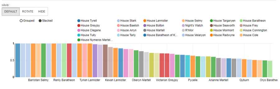
select name, house, popularity from character_deaths where House!="None" order by popularity desc limit 50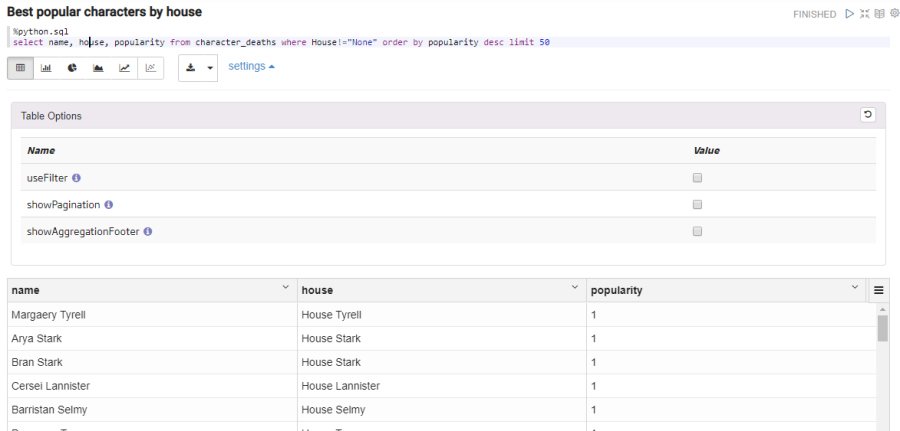

We can see the table-format view. But we can get a more interesting view with the bar graph: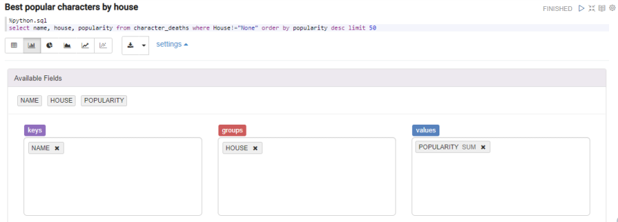


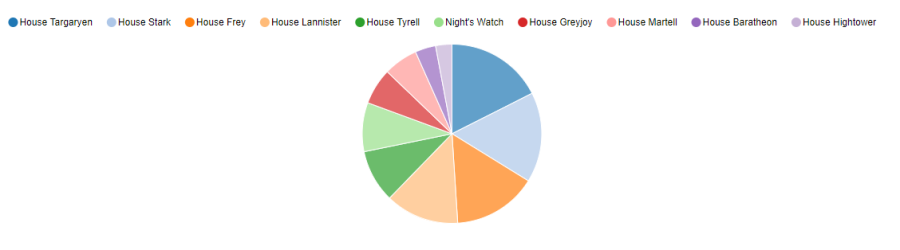
Or we can see the most popular houses in pie format:
%python.sql
select house, sum(popularity) as phouse from character_deaths where House!="None" group by House order by phouse desc limit 10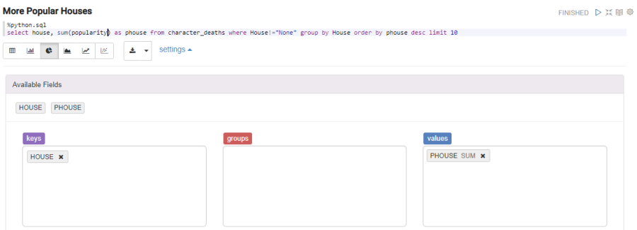


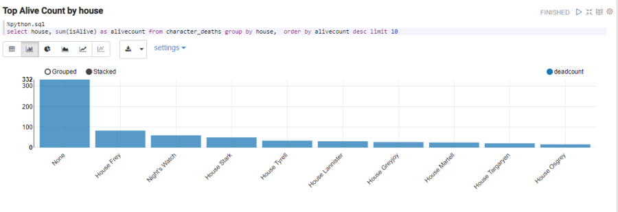
Or the top of houses with  more living people:
%python.sql
select house, sum(isAlive) as alivecount from character_deaths group by house order by alivecount desc limit 10

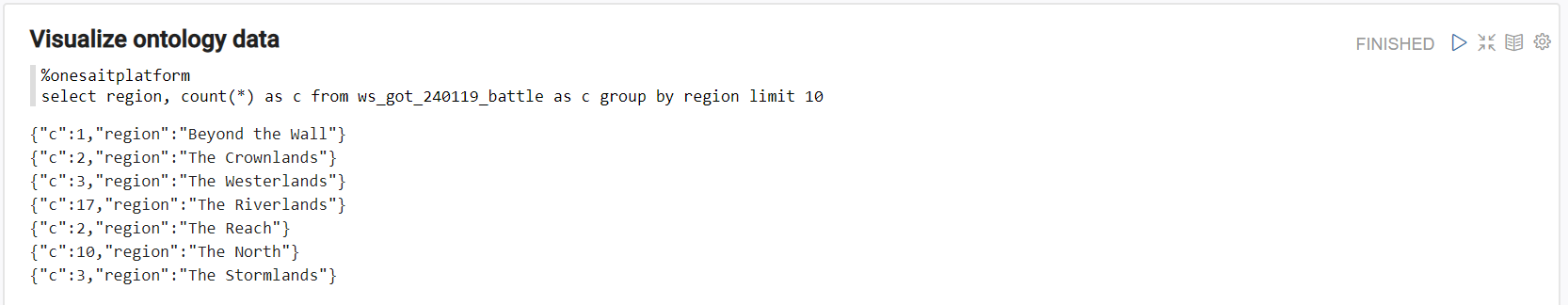
We can also do these queries or views directly against platform ontologies with the platform’s interpreter.

%onesaitplatform
select region, count(*) as c from {battle_ontology} as c group by region limit 10

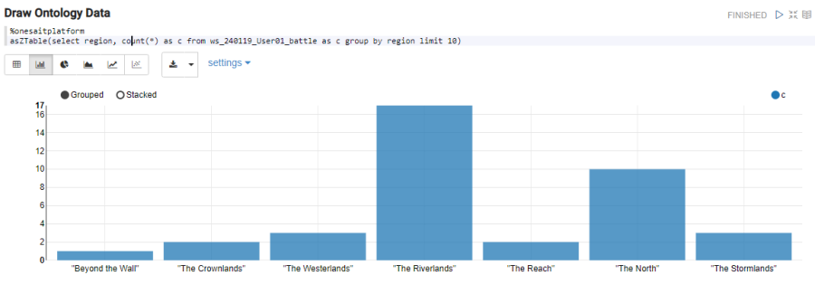
By using asZTable, the built-in view is started:

%onesaitplatform
asZTable(select region, count(*) as c from {battle_ontology} as c group by region limit 10)

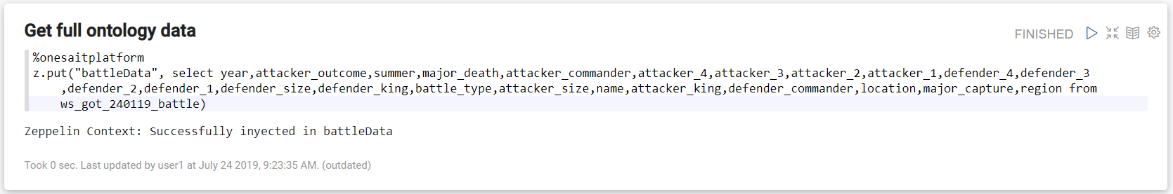
In the next section this will be useful, so we will save the pandas as data in the battle file ontology like this:
%onesaitplatform
z.put("battleData", select year,attacker_outcome,summer,major_death,attacker_commander,attacker_4,attacker_3,attacker_2,attacker_1,defender_4,defender_3,defender_2,defender_1,defender_size,defender_king,battle_type,attacker_size,name,attacker_king,defender_commander,location,major_capture,region from {battle_ontology})

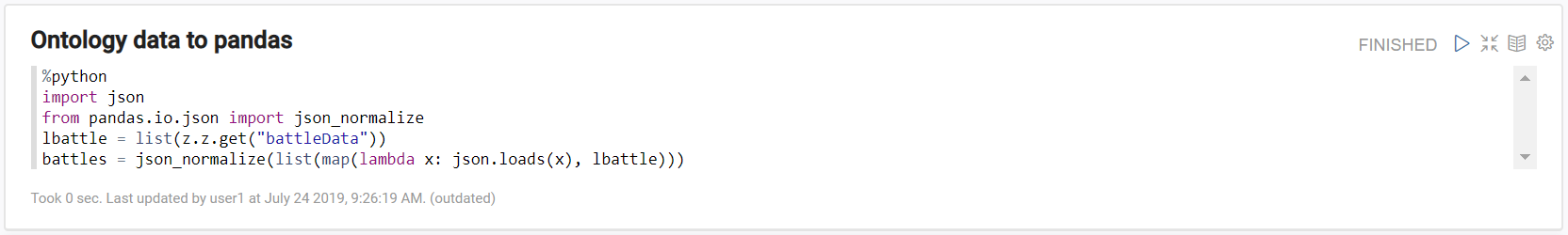
And later take it to the pandas dataframe: 
%python
import json
from pandas.io.json import json_normalize
lbattle = list(z.z.get("battleData"))
battles = json_normalize(list(map(lambda x: json.loads(x), lbattle)))

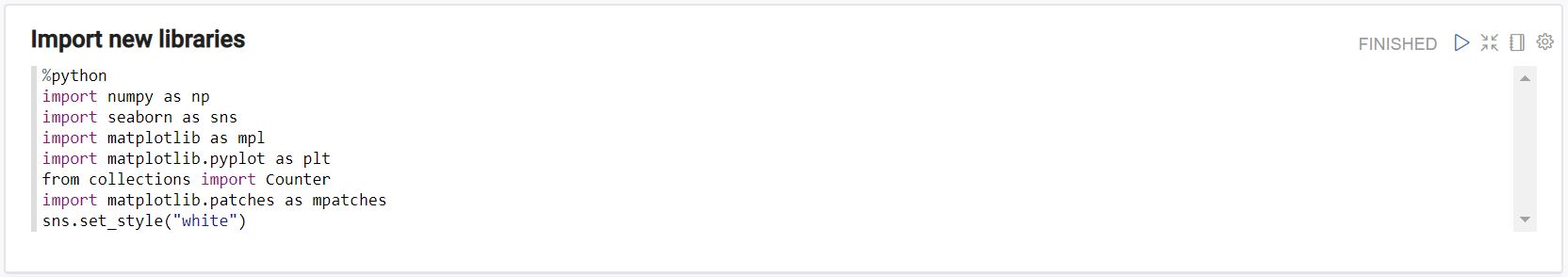
Lastly, to end the exploratory data part, we can use powerful graphs in the Python libraries such as matplotlib or seaborn.

These libraries will give us even more freedom tan the built-in view, at the expense of writing more code to build the goal graph.
Import new libraries
%python
import numpy as np
import seaborn as sns
import matplotlib as mpl
import matplotlib.pyplot as plt
from collections import Counter
import matplotlib.patches as mpatches
sns.set_style("white")

Generate new attributes
%python
character_predictions = character_deaths.copy(deep = True)
battles.loc[:, "defender_count"] = (4 - battles[["defender_1", "defender_2", "defender_3", "defender_4"]].isnull().sum(axis = 1))
battles.loc[:, "attacker_count"] = (4 - battles[["attacker_1", "attacker_2", "attacker_3", "attacker_4"]].isnull().sum(axis = 1))
battles.loc[:, "att_comm_count"] = [len(x) if type(x) == list else np.nan for x in battles.attacker_commander.str.split(",")]
character_predictions.loc[:, "no_of_books"] = character_predictions[[x for x in character_predictions.columns if x.startswith("book")]].sum(axis = 1)

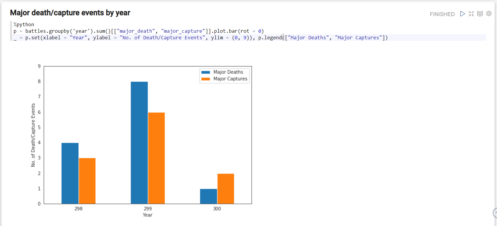
Major death/capture events by year
%python
p = battles.groupby('year').sum()[["major_death", "major_capture"]].plot.bar(rot = 0)
_ = p.set(xlabel = "Year", ylabel = "No. of Death/Capture Events", ylim = (0, 9)), p.legend(["Major Deaths", "Major Captures"])

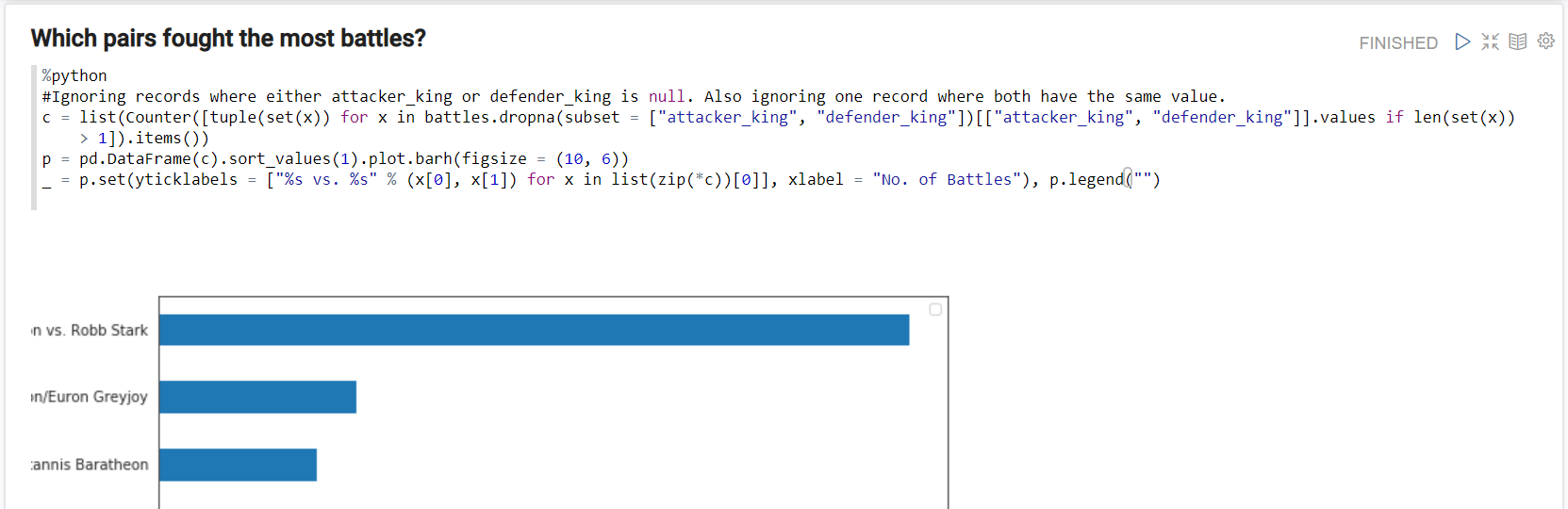
Which pairs fought the most battles?
%python
#Ignoring records where either attacker_king or defender_king is null. Also ignoring one record where both have the same value.
c = list(Counter([tuple(set(x)) for x in battles.dropna(subset = ["attacker_king", "defender_king"])[["attacker_king", "defender_king"]].values if len(set(x)) > 1]).items())
p = pd.DataFrame(c).sort_values(1).plot.barh(figsize = (10, 6))
_ = p.set(yticklabels = ["%s vs. %s" % (x[0], x[1]) for x in list(zip(*c))[0]], xlabel = "No. of Battles"), p.legend("")

How many commanders did armies of different kings have?
%python
p = sns.boxplot("att_comm_count", "attacker_king", data = battles, saturation = .6, fliersize = 10., palette = ["lightgray", sns.color_palette()[1], "grey", "darkblue"])
_ = p.set(xlabel = "No. of Attacker Commanders", ylabel = "Attacker King", xticks = range(8))

Lastly, we are going to generate several ML models with the idea of seeing the Python tools already integrated in the platform:
Data Cleansing

%python
#-------- Copy Again ----------

data = character_deaths.copy(deep = True)

#-------- culture induction -------
cult = {
    'Summer Islands': ['summer islands', 'summer islander', 'summer isles'],
    'Ghiscari': ['ghiscari', 'ghiscaricari',  'ghis'],
    'Asshai': ["asshai'i", 'asshai'],
    'Lysene': ['lysene', 'lyseni'],
    'Andal': ['andal', 'andals'],
    'Braavosi': ['braavosi', 'braavos'],
    'Dornish': ['dornishmen', 'dorne', 'dornish'],
    'Myrish': ['myr', 'myrish', 'myrmen'],
    'Westermen': ['westermen', 'westerman', 'westerlands'],
    'Westerosi': ['westeros', 'westerosi'],
    'Stormlander': ['stormlands', 'stormlander'],
    'Norvoshi': ['norvos', 'norvoshi'],
    'Northmen': ['the north', 'northmen'],
    'Free Folk': ['wildling', 'first men', 'free folk'],
    'Qartheen': ['qartheen', 'qarth'],
    'Reach': ['the reach', 'reach', 'reachmen'],
}

def get_cult(value):
    value = value.lower()
    v = [k for (k, v) in cult.items() if value in v]
    return v[0] if len(v) > 0 else value.title()

data.loc[:, "culture"] = [get_cult(x) for x in data.culture.fillna("")]

#-------- culture induction -------

data.drop(["name", "alive", "pred", "plod", "isAlive", "dateOfBirth", "dateoFdeath"], 1, inplace = True)

data.loc[:, "title"] = pd.factorize(data.title)[0]
data.loc[:, "culture"] = pd.factorize(data.culture)[0]
data.loc[:, "mother"] = pd.factorize(data.mother)[0]
data.loc[:, "father"] = pd.factorize(data.father)[0]
data.loc[:, "heir"] = pd.factorize(data.heir)[0]
data.loc[:, "house"] = pd.factorize(data.house)[0]
data.loc[:, "spouse"] = pd.factorize(data.spouse)[0]

data.fillna(value = -1, inplace = True)
''' $$ The code below usually works as a sample equilibrium. However in this case,
 this equilibirium actually decrease our accuracy, all because the original 
prediction data was released without any sample balancing. $$

data = data[data.actual == 0].sample(350, random_state = 62).append(data[data.actual == 1].sample(350, random_state = 62)).copy(deep = True).astype(np.float64)

'''
Y = data.actual.values

Odata = data.copy(deep=True)

data.drop(["actual"], 1, inplace = True)

Feature Correlation
%python
sns.heatmap(data.corr(),annot=True,cmap='RdYlGn',linewidths=0.2) #data.corr()-->correlation matrix
fig=plt.gcf()
fig.set_size_inches(30,20)
plt.show()

RandomForest (over fit)
%python
data.drop(["sNo"], 1, inplace = True)
''' ATTENTION: This rf algorithm achieves 99%+ accuracy, this is because the \
original predictor-- the document releaser use exactly the same algorithm to predict!
'''
from sklearn.ensemble import RandomForestClassifier

random_forest = RandomForestClassifier(n_estimators=100)
random_forest.fit(data, Y)
print('RandomForest Accuracy：(original)\n',random_forest.score(data, Y))

DecisionTree
%python
from sklearn.tree import DecisionTreeClassifier
DT=DecisionTreeClassifier()
DT.fit(data,Y)
print('DecisionTree Accuracy：(original)\n',DT.score(data, Y))

SVC
%python
from sklearn.svm import SVC, LinearSVC
svc = SVC()
svc.fit(data, Y)
print('SVC Accuracy：\n',svc.score(data, Y))

LogisticRegression
%python
from sklearn.linear_model import LogisticRegression
LR = LogisticRegression()
LR.fit(data, Y)
print('LogisticRegression Accuracy：\n',LR.score(data, Y))

KNN
%python
from sklearn.neighbors import KNeighborsClassifier
knn = KNeighborsClassifier(n_neighbors = 3)
knn.fit(data, Y)
print('kNN Accuracy：\n',knn.score(data, Y))

NaiveBayes Gaussian
%python
from sklearn.naive_bayes import GaussianNB
gaussian = GaussianNB()
gaussian.fit(data, Y)
print('gaussian Accuracy：\n',gaussian.score(data, Y))

RandomForest with CrossValidation
%python
from sklearn.model_selection import cross_validate
from sklearn.model_selection import KFold
from sklearn.model_selection import cross_val_score
from sklearn.ensemble import RandomForestClassifier
predictors=['title', 'culture', 'mother', 'father', 'heir', 'house', 'spouse', 'male', 'book1', 'book2', 'book3', 'book4', 'book5', 'isAliveFather', 'isAliveMother', 'isAliveHeir', 'isAliveSpouse', 'isMarried', 'isNoble', 'age', 'numDeadRelations', 'boolDeadRelations', 'isPopular', 'popularity']
alg=RandomForestClassifier(random_state=1,n_estimators=150,min_samples_split=12,min_samples_leaf=1)
kf=KFold(n_splits=3,random_state=1)
kf=kf.get_n_splits(Odata.shape[0])
scores=cross_val_score(alg,Odata[predictors],Odata["actual"],cv=kf)
print('RandomForest Accuracy：\n',scores.mean())

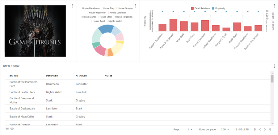
4. Viewing the data using the platform's dashboards

Our goal in this section will be using the dashboard engine integrated in the platform. We recommend using Google Chrome because the web engine is optimized for it.

We will generate a view, with data loaded from the previous steps. These generated dashboards can be shared with different users, customized, be made public and many other options.
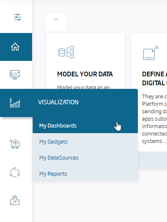
Firstly, with a logged user, we will create our first dashboard. To do this, we go to My Dashboards in the menu Visualizations, and then we click Create Dashboard.

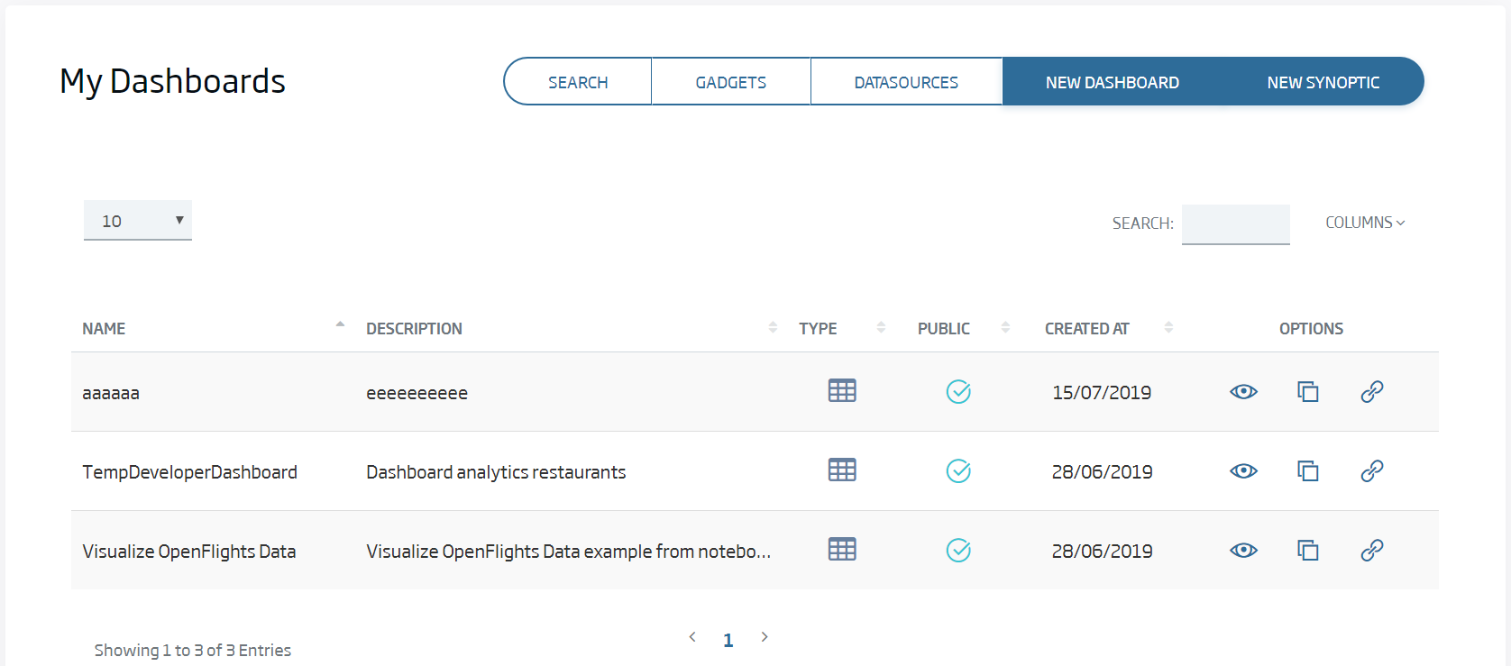
We can see that, we enter the menu, we can see the public dashboards, our own dashboards, and those we are allowed to see.

There, we give a new to our new dashboard:
ws_got_{date}_{User01}_Visualization

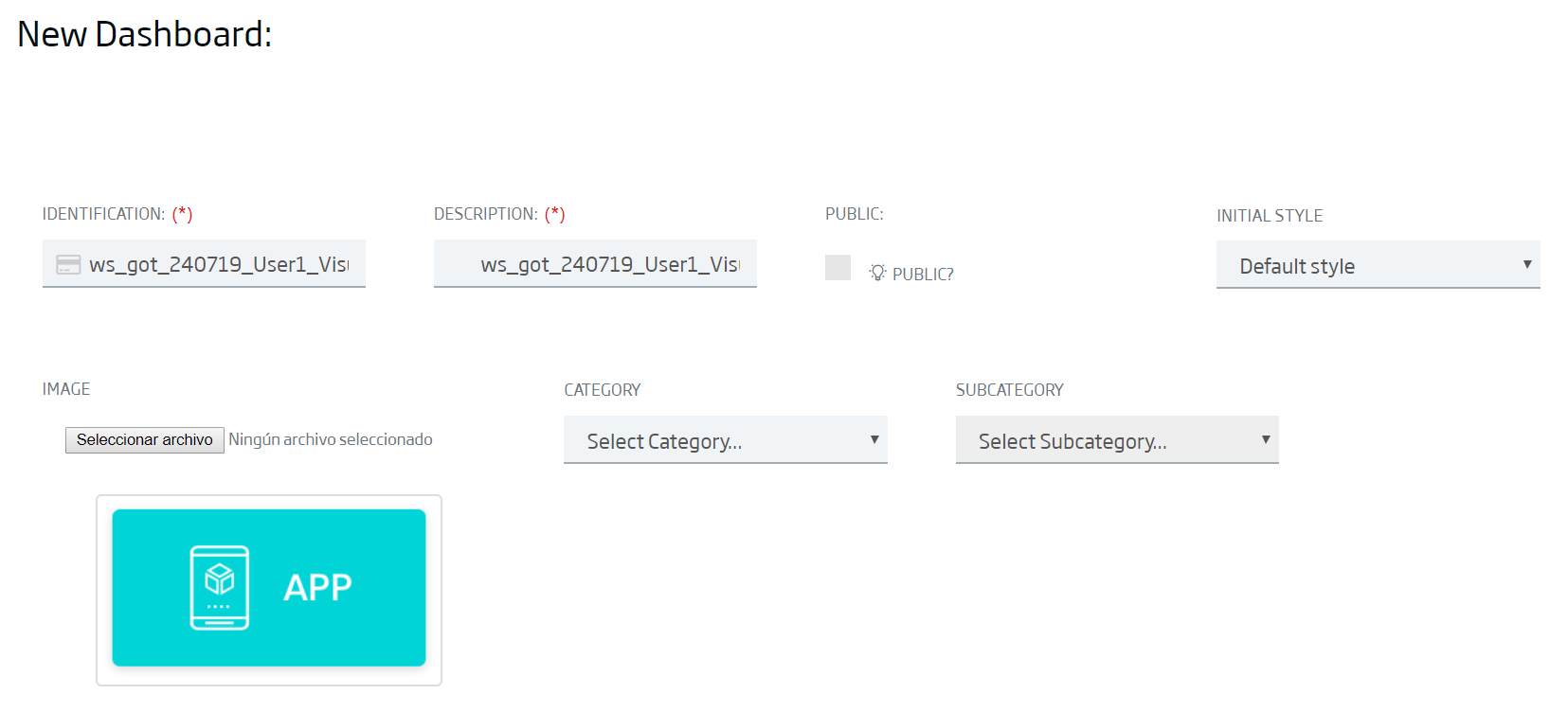
Lastly, without any other change, we click "New" and our dashboard is already created. We can verify it, because we will reach an empty canvas on which we would include elements called "gadgets" that will recover data directly from the ontologies.

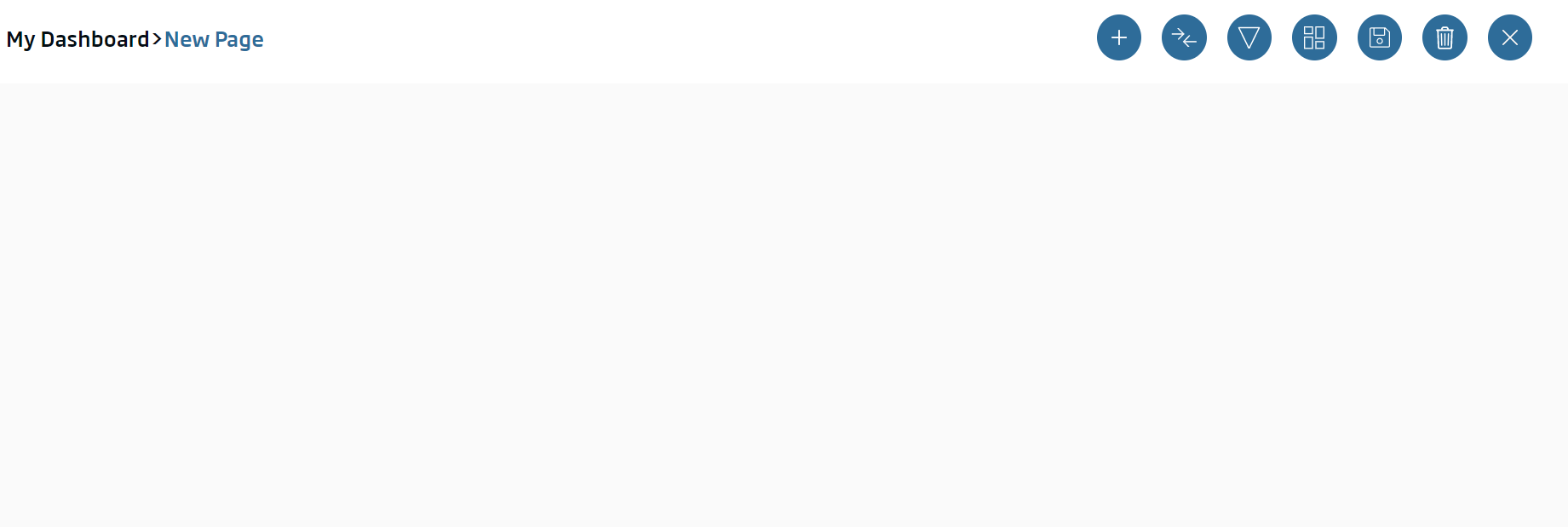
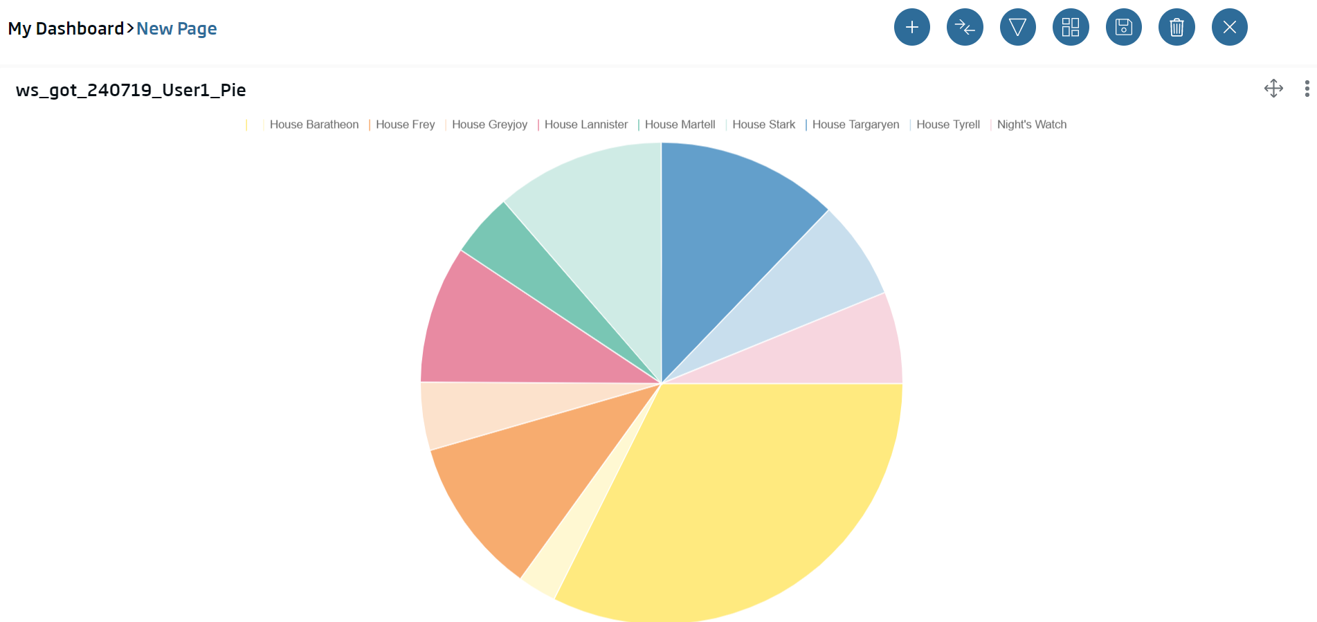
We are going to create our first gadget. In this case, it will be a Pie gadget to see the popularity distribution among the different houses.

This gadget will become the filter over other future gadgets in the dashboard.
To do this, we will add a new gadget using the  button, in the upper right side. We see there is a band with the available gadgets in the platform:

 
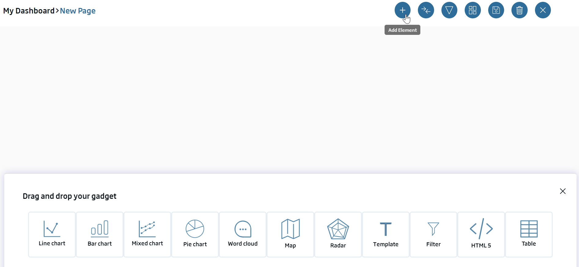
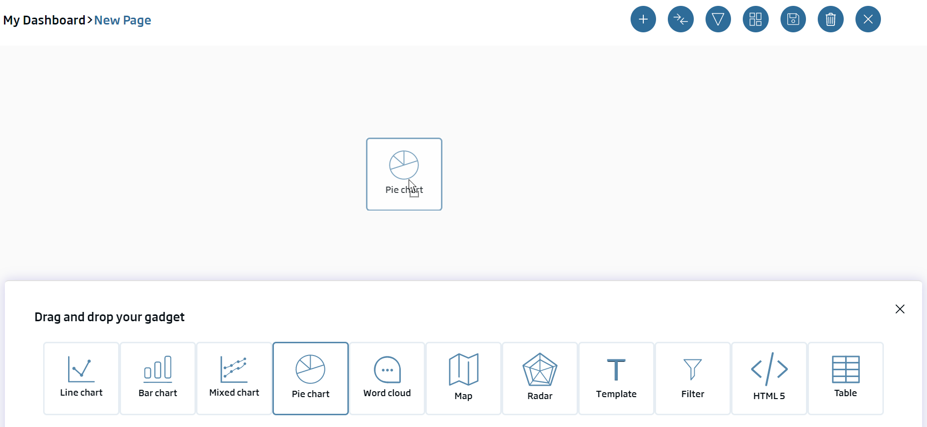
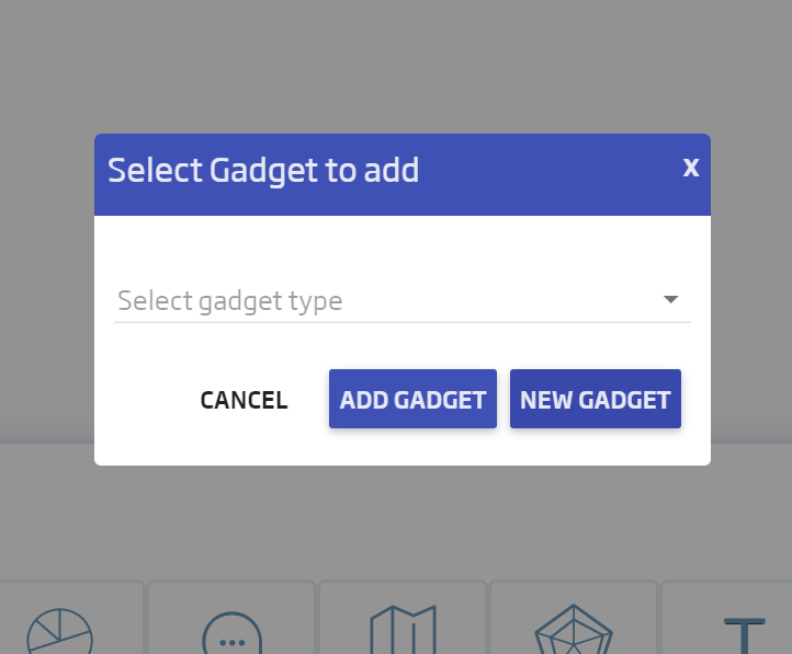
We drag and drop the gadget type (Pie chart) within the canvas, to the area we want to paint it. When we drop, we will see the following pop-up, where we will select "New Gadget" because we have no previously created pie gadget.

 
We will see the gadget creation form, where:  
Nombre: ws_got_240119_User01_pie
Ontology or Datasource: (our deaths ontology)

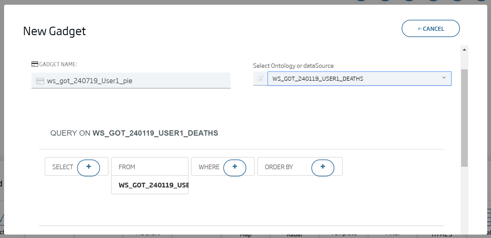
As we can see, we will be provided a default query.

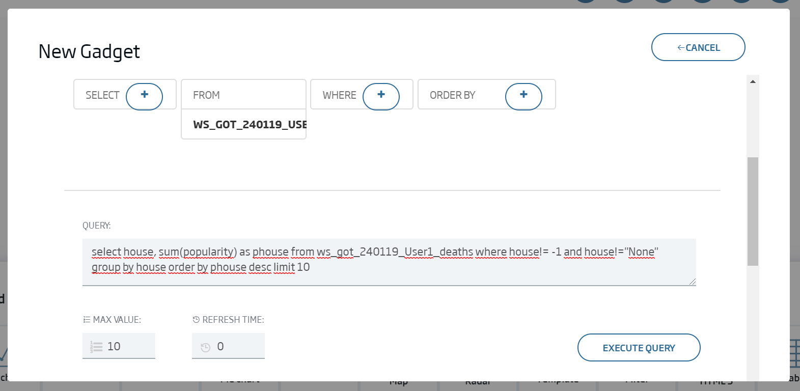
We will first leave Max Values as 10 and, as we want to see the popularity of houses, we will use this query:
select house, sum(popularity) as phouse from {ontología cdeaths} where house!= -1 and house!="None" group by house order by phouse desc limit 10
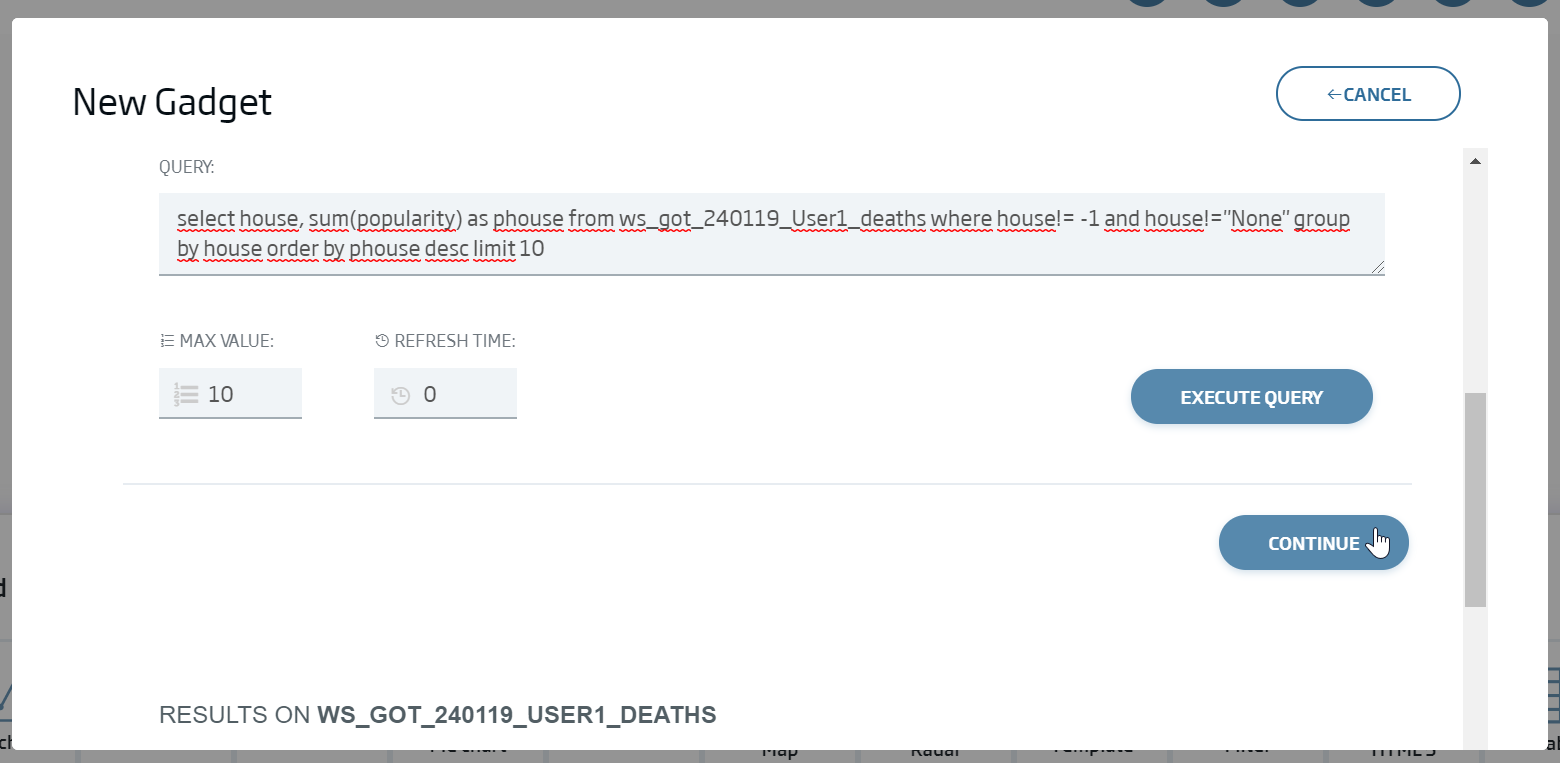
So we will have grouped the houses by their total popularity. If we execute it in the form, we can see the results.

 
We click "Continue".

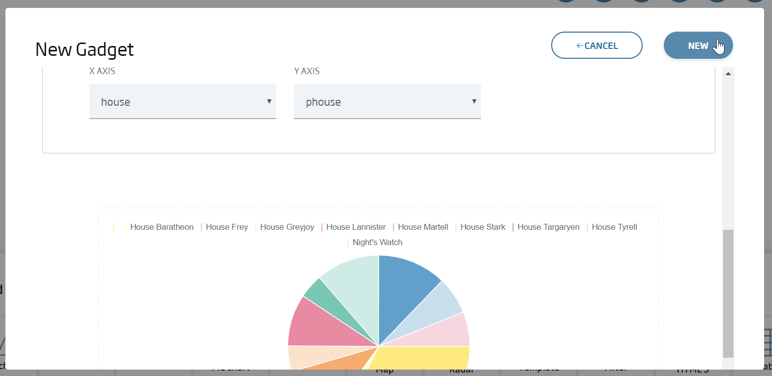
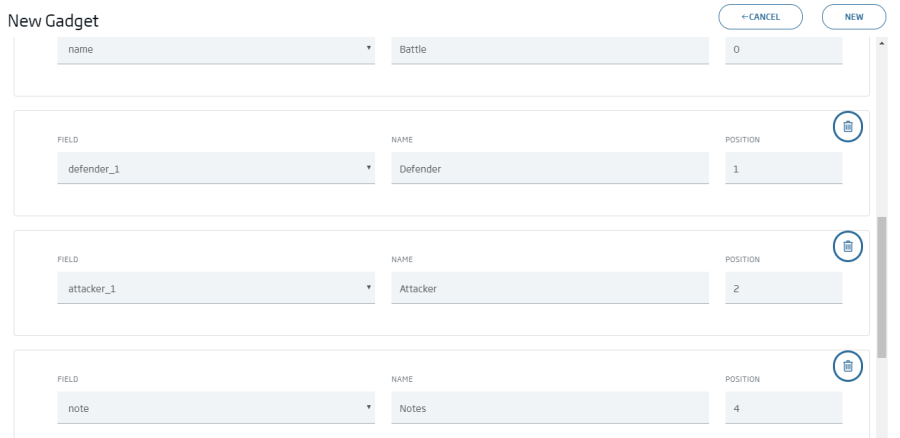
Lastly, we select the fields for our pie:

X Axis: house

Y Axis: phouse

We select New.

 
 
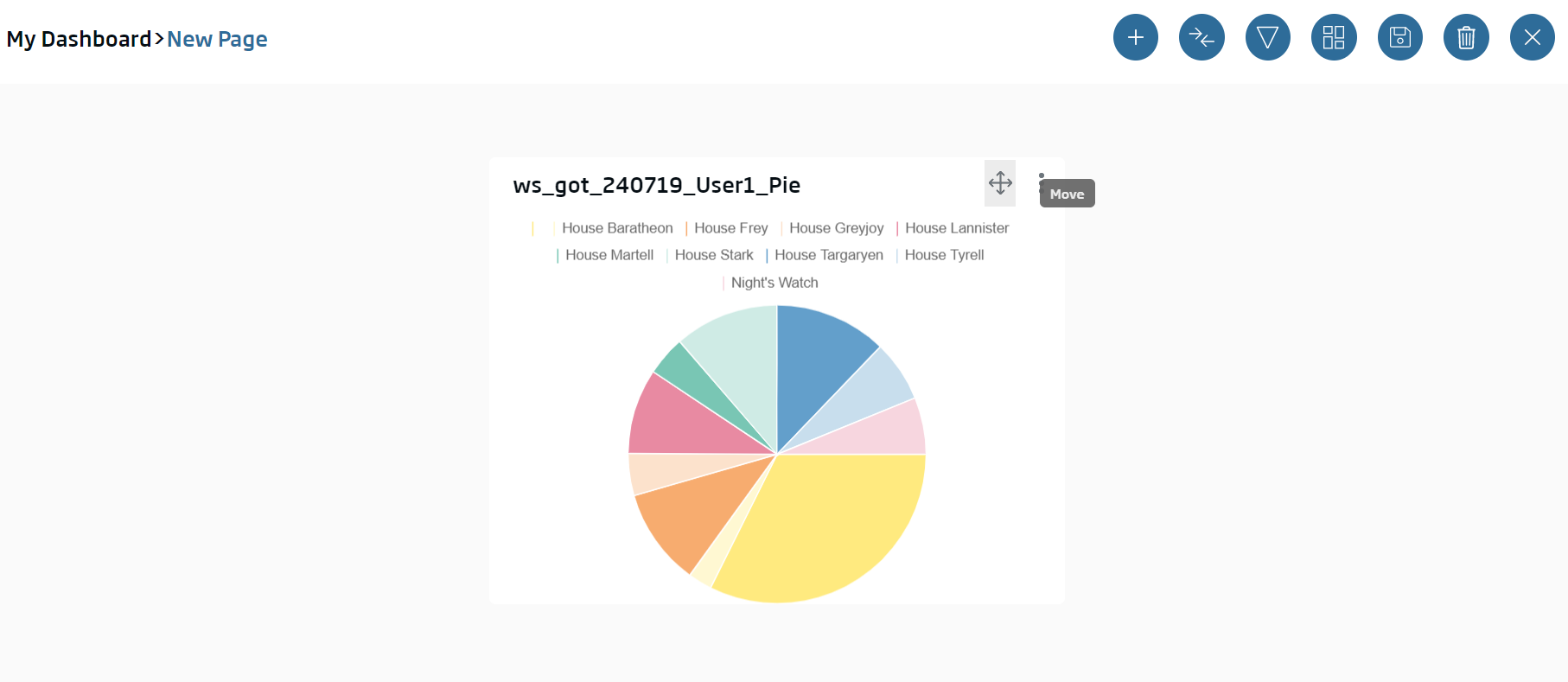
Through its borders, we can re-dimension the element or move it in the canvas using the header arrows.

We will swiftly create a couple more gadgets:
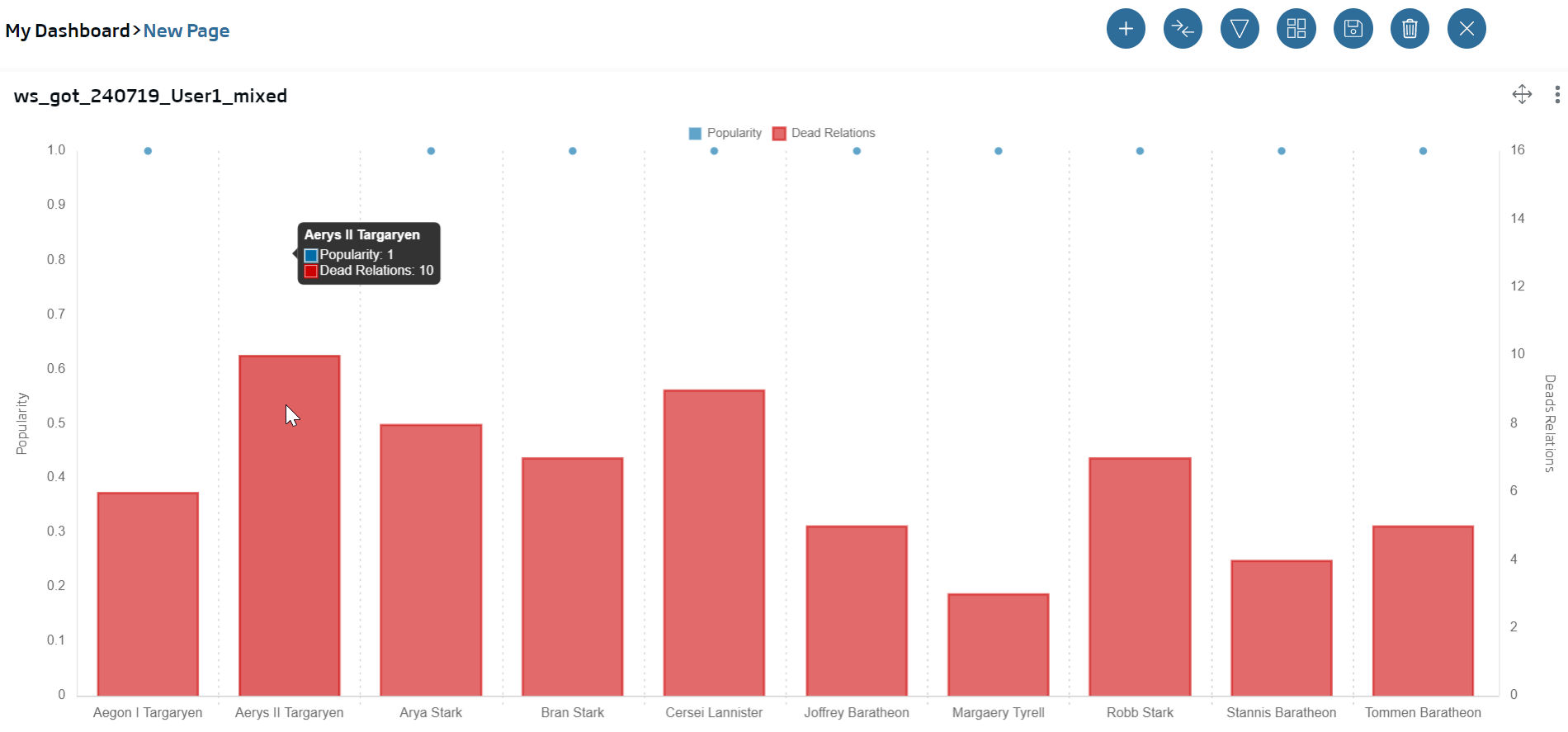
Firstly, a Mixed one where we will see the characters’ individual popularity:
Name: ws_got_{date}_{user}_mixed

select * from {ontología cdeaths} order by popularity desc limit 10

 
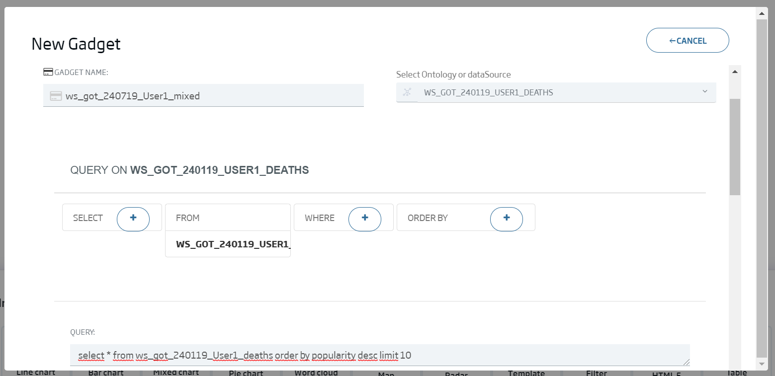
We click Continue and we write the configuration we can see in this image:

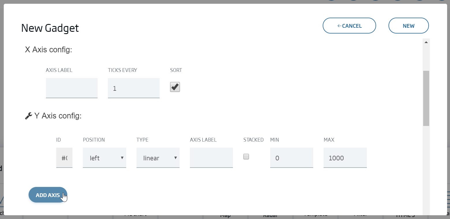
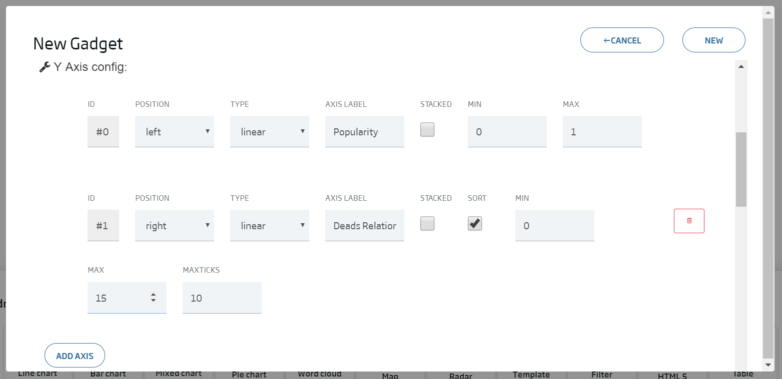
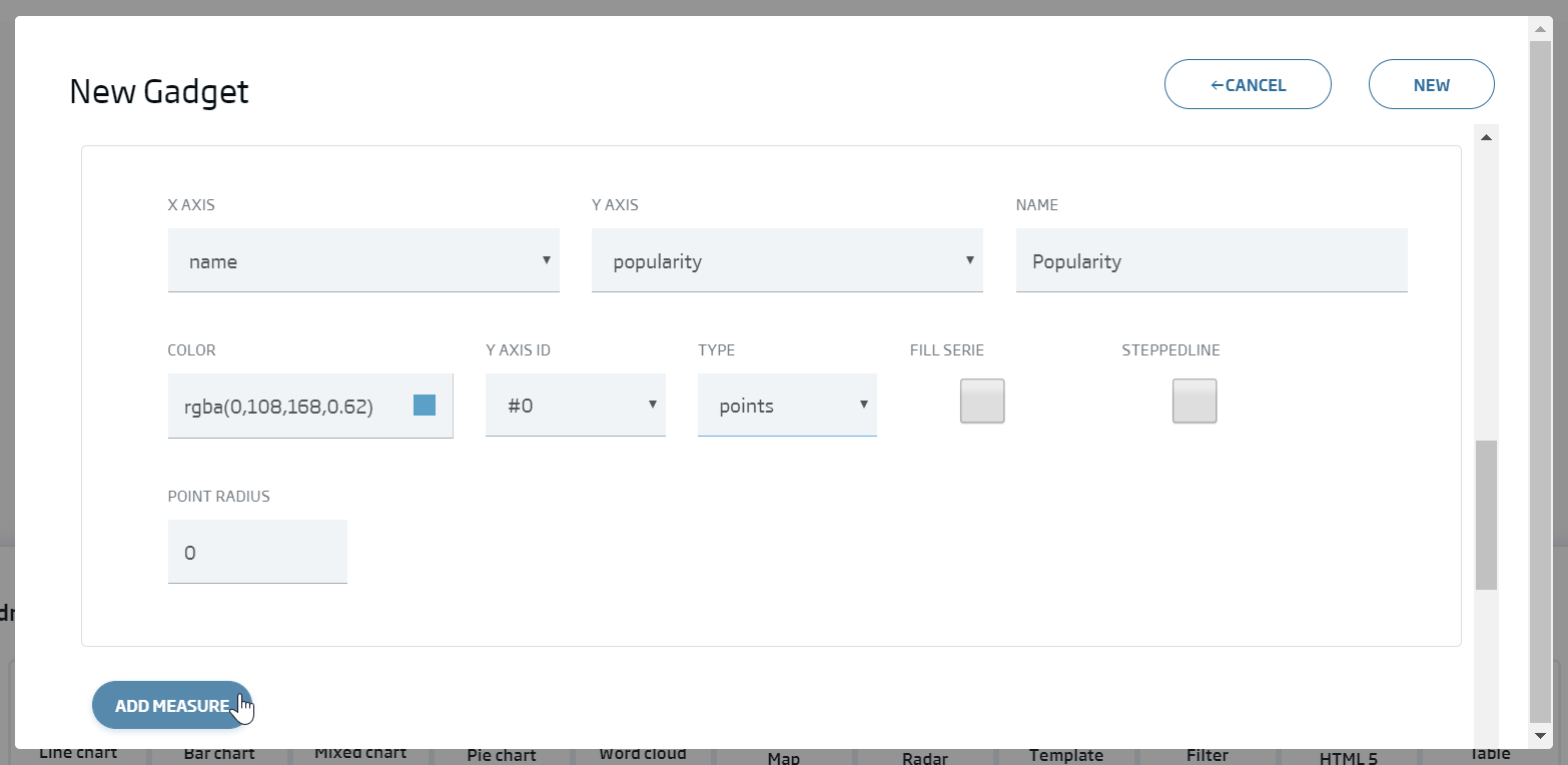
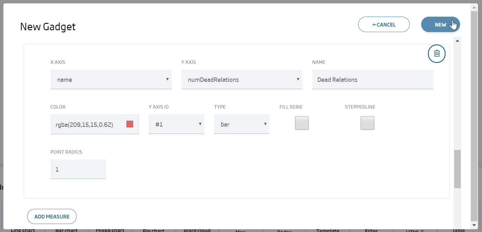
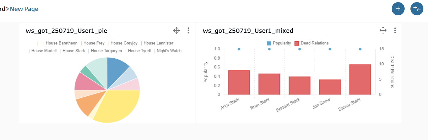
We will finally see the following graph:

 
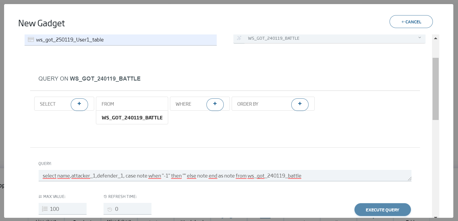
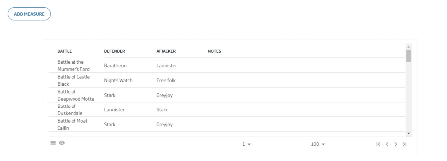
The second one, a table to be used as battle logbook:
ws_got_240119_User01_table
Query: select name,attacker_1,defender_1, case note when "-1" then "" else note end as note from {ontología battle} 

Placing everything in place, our dashboard should look like this: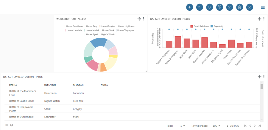

Let’s link these gadgets up there because, as we can see, we can filter the characters to the right by the house at a datasource level. To do this, we will use the   (Datalink):

 
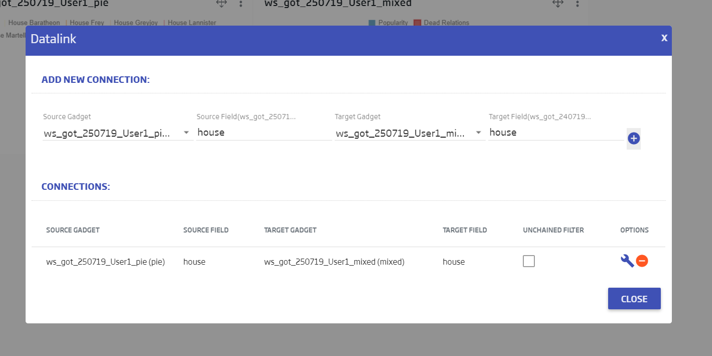
We specify that our Pie is the source and our Mixed is the target. The connecting field will be house, for both of them:

 
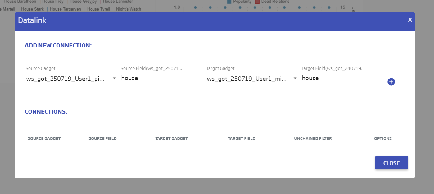
We click  to add the connection and, when we close, any click in the pie will filter the Mixed Gadget.

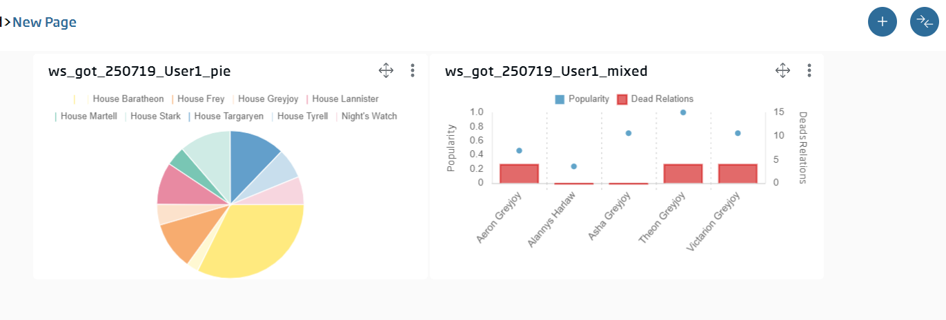
With a little bit of embellishment, the dashboard can give a final result like this one: